Pinhole Camera Model
Table of contents
- Overview
- 13. Complete intrinsic matrix
- 14. Connection between normalized and pixel interaction matrices
- 3. Why “calibrated mapping with convenient signs”?
- 4. Why does the virtual image plane work physically?
- 5. Is the camera manufacturer doing the sign flip?
- 9. Physical focal length \(f\)
- 10. Meaning of \(f_x\) and \(f_y\)
- 11. Numerical conversion example
- 12. Why use two focal lengths instead of one?
Overview
The pinhole camera model describes perspective projection from a 3D point to a 2D image. Let a point expressed in the camera frame be \(P_c=[X,Y,Z]^T\), with the camera center at the origin and the optical axis aligned with the positive \(Z\)-axis. Although a physical sensor lies behind the pinhole and forms an inverted image, an equivalent virtual image plane at \(Z=f\) is usually placed in front of it to simplify the geometry.
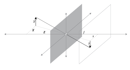
By similar triangles, the ray from \(P_c\) through the camera center intersects the virtual image plane at
\[\begin{bmatrix} X \\ Y \\ Z \end{bmatrix} \longmapsto \begin{bmatrix} fX/Z \\ fY/Z \\ f \end{bmatrix}.\]Dropping the fixed third coordinate gives the image-plane location \((fX/Z,fY/Z)\). Dividing it by \(f\) gives the normalized image coordinates used later in this chapter:
\[x=\frac{X}{Z}, \qquad y=\frac{Y}{Z}.\]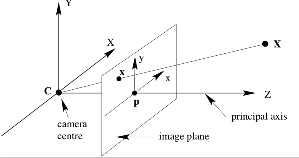
In this geometry:
-
the camera center \(C\) is the center of projection;
-
the image plane is the plane at \(Z=f\);
-
the principal axis is perpendicular to the image plane and passes through \(C\);
-
the principal point is where the principal axis intersects the image plane;
-
the principal plane passes through \(C\) and is parallel to the image plane.
If the same point is initially expressed in the world frame as \(P_w=[X_w,Y_w,Z_w,1]^T\), the extrinsic matrix \([R\mid t]\) first rotates and translates it into the camera frame. The intrinsic matrix \(K\) then converts the camera-frame coordinates into homogeneous pixel coordinates:
\[P_c = \begin{bmatrix} X \\ Y \\ Z \end{bmatrix} = [R\mid t]P_w,\] \[Z \begin{bmatrix} u \\ v \\ 1 \end{bmatrix} = KP_c = K[R\mid t]P_w = PP_w, \qquad P=K[R\mid t].\]Thus, \([R\mid t]\) determines where the point is relative to the camera, while \(K\) determines where its viewing ray appears in the pixel coordinate system. Together they form the \(3\times4\) camera projection matrix \(P\).
13. Complete intrinsic matrix
The general intrinsic matrix is
\[K= \begin{bmatrix} f_x & s & c_x \\ 0 & f_y & c_y \\ 0 & 0 & 1 \end{bmatrix},\]where:
-
\(f_x,f_y\) are focal lengths in pixels;
-
\(c_x,c_y\) are the principal point in pixels;
-
\(s\) is the skew coefficient.
For most modern cameras,
\[s\approx0,\]so
\[K= \begin{bmatrix} f_x & 0 & c_x \\ 0 & f_y & c_y \\ 0 & 0 & 1 \end{bmatrix}.\]The homogeneous projection is
\[Z \begin{bmatrix} u \\ v \\ 1 \end{bmatrix} = K \begin{bmatrix} X \\ Y \\ Z \end{bmatrix}.\]Expanding,
\[Zu=f_xX+c_xZ,\] \[Zv=f_yY+c_yZ.\]Dividing by \(Z\) gives
\[\boxed{ u=f_x\frac{X}{Z}+c_x }, \qquad \boxed{ v=f_y\frac{Y}{Z}+c_y }.\]14. Connection between normalized and pixel interaction matrices
The normalized feature is
\[s_n= \begin{bmatrix} x \\ y \end{bmatrix},\]while the pixel feature is
\[s_p= \begin{bmatrix} u \\ v \end{bmatrix} = \begin{bmatrix} f_xx+c_x \\ f_yy+c_y \end{bmatrix}.\]Differentiate:
\[\dot{u}=f_x\dot{x}, \qquad \dot{v}=f_y\dot{y}.\]Therefore,
\[\begin{bmatrix} \dot{u} \\ \dot{v} \end{bmatrix} = \begin{bmatrix} f_x & 0 \\ 0 & f_y \end{bmatrix} \begin{bmatrix} \dot{x} \\ \dot{y} \end{bmatrix}.\]If
\[\dot{s}_n=L_n\nu_c,\]then
\[\dot{s}_p = \begin{bmatrix} f_x & 0 \\ 0 & f_y \end{bmatrix} L_n\nu_c.\]Hence,
\[\boxed{ L_{\mathrm{pixel}} = \begin{bmatrix} f_x & 0 \\ 0 & f_y \end{bmatrix} L_n }.\]With nonzero skew, the multiplier becomes
\[\begin{bmatrix} f_x & s \\ 0 & f_y \end{bmatrix}.\]This is why focal lengths appear when the lecture moves from normalized coordinates to pixel coordinates.
3. Why “calibrated mapping with convenient signs”?
This sentence is easy to misunderstand.
It does not mean:
The software changes the real image into the virtual image.
It means:
The camera system provides a calibrated mathematical relationship:
\[(X,Y,Z)\rightarrow(u,v)\]that already uses a chosen coordinate convention.
The calibration gives you:
\[K= \begin{bmatrix} f_x & 0 & c_x \\ 0 & f_y & c_y \\ 0 & 0 & 1 \end{bmatrix}\]and the projection model:
\[u=f_x\frac{X}{Z}+c_x\] \[v=f_y\frac{Y}{Z}+c_y\]This is the “calibrated mapping.”
What does calibration actually do?
Suppose you have a chessboard.
You know its real 3D points:
\[P_w\]You detect their image locations:
\[(u,v)\]The calibration algorithm finds:
\[K,R,t\]such that:
\[Z \begin{bmatrix} u \\ v \\ 1 \end{bmatrix} = K \begin{bmatrix} R \mid t \end{bmatrix} \begin{bmatrix} X_w \\ Y_w \\ Z_w \\ 1 \end{bmatrix}\]The camera does not tell you:
“The physical image plane is virtual.”
Instead, calibration says:
“Given this pixel coordinate system, this \(K\) makes the projection equations correct.”
4. Why does the virtual image plane work physically?
This is the key idea:
A camera image is fundamentally a set of rays.
The 3D point:
\[P_c= \begin{bmatrix} X \\ Y \\ Z \end{bmatrix}\]creates a ray:
\[\lambda \begin{bmatrix} X \\ Y \\ Z \end{bmatrix}\]The physical sensor and virtual plane are just two different ways of selecting a point on this same ray.
Physical plane:
\[Z=-f\]gives:
\[x=-f\frac{X}{Z}\]Virtual plane:
\[Z=f\]gives:
\[x=f\frac{X}{Z}\]They differ only by a sign.
The ray itself did not change.
Why does OpenCV choose virtual coordinates?
Because it gives nicer properties:
Property 1
Points in front of the camera have:
\[Z>0\]instead of:
\[Z<0\]Property 2
A point on the right gives:
\[u>c_x\]which matches image intuition.
Property 3
The intrinsic matrix contains positive focal lengths:
\[f_x>0\]instead of negative values.
This makes optimization and calibration much easier.
5. Is the camera manufacturer doing the sign flip?
Partially, but not exactly.
There are two separate things:
Optical formation
The lens physically forms an inverted image.
Digital image representation
The camera electronics output an image array.
The camera driver chooses:
-
where pixel \((0,0)\) is,
-
whether rows increase downward,
-
whether columns increase rightward.
The final digital image coordinate system is what OpenCV sees.
So the manufacturer or camera firmware may indeed perform operations like:
-
flipping,
-
rotating,
-
demosaicing,
-
correcting sensor orientation.
But the important point is:
OpenCV calibration is performed on the final digital image coordinates.
The intrinsic matrix \(K\) already describes the mapping between 3D rays and those pixels.
9. Physical focal length \(f\)
The physical focal length is a length, commonly measured in millimetres:
\[f_{\mathrm{physical}} \quad [\mathrm{mm}].\]For example,
\[f_{\mathrm{physical}}=4\ \mathrm{mm}.\]Pixel coordinates \(u\) and \(v\) are measured in pixels, so a focal length expressed in millimetres cannot be inserted directly into
\[u=f_x\frac{X}{Z}+c_x.\]It must first be converted into pixel units.
10. Meaning of \(f_x\) and \(f_y\)
The quantities \(f_x\) and \(f_y\) are focal lengths measured in horizontal and vertical pixels:
\[f_x\quad[\mathrm{pixels}], \qquad f_y\quad[\mathrm{pixels}].\]Let the physical pixel pitches be
\[d_x\quad[\mathrm{mm/pixel}], \qquad d_y\quad[\mathrm{mm/pixel}].\]Then
\[\boxed{ f_x=\frac{f_{\mathrm{physical}}}{d_x} }, \qquad \boxed{ f_y=\frac{f_{\mathrm{physical}}}{d_y} }.\]Equivalently, define pixel densities
\[m_x=\frac{1}{d_x} \quad[\mathrm{pixels/mm}], \qquad m_y=\frac{1}{d_y} \quad[\mathrm{pixels/mm}].\]Then
\[\boxed{ f_x=f_{\mathrm{physical}}m_x }, \qquad \boxed{ f_y=f_{\mathrm{physical}}m_y }.\]Some texts use \(\alpha_x\) and \(\alpha_y\) instead of \(f_x\) and \(f_y\):
\[\alpha_x=fm_x, \qquad \alpha_y=fm_y.\]These quantities have the same role as the OpenCV notation \(f_x,f_y\).
11. Numerical conversion example
Suppose
\[f_{\mathrm{physical}}=4\ \mathrm{mm},\]with pixel pitches
\[d_x=0.005\ \mathrm{mm/pixel}, \qquad d_y=0.0048\ \mathrm{mm/pixel}.\]Then
\[f_x=\frac{4}{0.005}=800\ \mathrm{pixels},\]and
\[f_y=\frac{4}{0.0048}\approx833.33\ \mathrm{pixels}.\]The pixel projection is therefore
\[u=800\frac{X}{Z}+c_x,\] \[v=833.33\frac{Y}{Z}+c_y.\]Because \(X\) and \(Z\) use the same length unit,
\[\frac{X}{Z}\]is dimensionless. Consequently, \(f_x(X/Z)\) has units of pixels, matching \(u\).
12. Why use two focal lengths instead of one?
There are several practical reasons.
Different pixel pitch
The horizontal and vertical physical pixel spacing can differ:
\[d_x\neq d_y.\]Then
\[f_x\neq f_y.\]Image resizing
If an image is resized with horizontal and vertical scale factors \(r_x,r_y\), the intrinsic parameters change as
\[f_x'=r_xf_x, \qquad f_y'=r_yf_y,\] \[c_x'=r_xc_x, \qquad c_y'=r_yc_y.\]Calibration estimates the pixel geometry directly
In practice, \(f_x\) and \(f_y\) are normally estimated directly through calibration, rather than reconstructed from nominal lens focal length and sensor pitch. This captures small manufacturing and processing differences. For nominally square pixels,
\[f_x\approx f_y,\]but they need not be forced to be exactly equal.
Reference: