
From Q-Learning to Deep Q-Learning and Deep Deterministic Policy Gradient (DDPG)
Published:
Q-learning, an off-policy reinforcement learning algorithm, uses the Bellman equation to iteratively update state-action values, helping an agent determine the best actions to maximize cumulative rewards. Deep Q-learning improves upon Q-learning by leveraging deep Q network (DQN) to approximate Q-values, enabling it to handle continuous state spaces but it is still only suitable for discrete action spaces. Further advancement, Deep Deterministic Policy Gradient (DDPG), combines Q-learning’s principles with policy gradients, making it also suitable for continuous action spaces. This blog starts by discussing the basic components of reinforcement learning and gradually explore how Q-learning evolves into DQN and DDPG, with application for solving the cartpole environment in Isaac Gym simulator. Corresponding code can be found at this repository.
Reinforcement Learning Overview
The goal of reinforcement learning is to train an agent to interact with an environment to maximize cumulative rewards over time. Unlike supervised learning, RL does not rely on labeled data but instead learns from feedback in the form of rewards or penalties.
In contrast to typical optimal control problems, which use differential equations to describe system dynamics, reinforcement learning problems are typically modeled as MDPs, which can sometimes be beneficial in terms of taking model uncertainty into account. An MDP is defined by the tuple \((S, A, P, R, γ)\):
- \(S\): Set of states.
- \(A\): Set of actions.
- \(P(s' \mid s, a)\): Transition probability to \(s'\) given state \(s\) and action \(a\).
- \(R(s, a)\): Reward function for taking action \(a\) in state \(s\).
- \(γ\): Discount factor to prioritize short-term vs. long-term rewards.
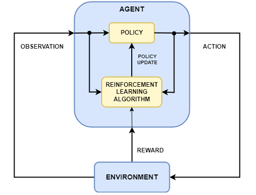
The picture above shows a general representation of reinforcement learning scenario and illustrate the necessary component which includes:
- Agent: Learns the policy (π) to maximize rewards.
- Environment: The system the agent interacts with.
- Reward Signal: Feedback to guide the agent.
- Policy: Maps states to actions (\(\pi (a \mid s)\)).
- Value / Q Function: Estimates the “goodness” of states or state-action pairs.
Bellman Equation
The Bellman equation is the cornerstone of reinforcement learning, describing the relationship between the value of a state and the values of its successor states. It is a recursive decomposition of the value function.
The Bellman equation expresses \(V^\pi(s)\) recursively:
\[V^\pi(s) = \sum_a \pi(a \mid s) \sum_{s'} P(s' \mid s, a) \left[ R(s, a) + \gamma V^\pi(s') \right]\]Where:
- \(P(s' \mid s, a)\): Transition probability to state \(s'\) after taking action \(a\).
- \(R(s, a)\): Immediate reward.
The value of a state \(s\) under a policy \(\pi\) is the expected cumulative reward starting from \(s\), following \(\pi\):
\[V^\pi(s) = \mathbb{E}_\pi \left[ \sum_{t=0}^\infty \gamma^t r_t \; \middle| \; s_0 = s \right]\]Here:
- \(r_t\): Reward at time step \(t\).
- \(\gamma\): Discount factor (\(0 \leq \gamma \leq 1\)).
- \(\pi(a \mid s)\): Probability of taking action \(a\) in state \(s\) under policy \(\pi\).
Bellman Optimality Equation (Optimal Value Function)
For the optimal policy \(\pi^*\), the Bellman equation becomes:
\[V^*(s) = \max_a \sum_{s'} P(s' \mid s, a) \left[ R(s, a) + \gamma V^*(s') \right]\]The Bellman equation provides the foundation for dynamic programming methods like value iteration and policy iteration.
Q Function and Value Function
The value function and Q-function represent different perspectives on evaluating the quality of states and actions:
- Value Function (\(V^\pi(s)\))
Measures the expected cumulative reward starting from a state \(s\) and following a policy \(\pi\):
\[V^\pi(s) = \mathbb{E}_\pi \left[ \sum_{t=0}^\infty \gamma^t r_t \; \middle| \; s_0 = s \right]\]- Q-Function (\(Q^\pi(s, a)\))
Extends the value function by also considering the action \(a\) taken in \(s\) before following \(\pi\):
\[Q^\pi(s, a) = \mathbb{E}_\pi \left[ r_0 + \gamma V^\pi(s_1) \; \middle| \; s_0 = s, a_0 = a \right]\]Or equivalently:
\[Q^\pi(s, a) = R(s, a) + \gamma \sum_{s'} P(s' \mid s, a) V^\pi(s').\]- Relationship Between \(Q(s, a)\) and \(V(s)\)
The value function can be derived from the Q-function:
\[V^\pi(s) = \sum_a \pi(a \mid s) Q^\pi(s, a).\]For the optimal policy:
\[V^*(s) = \max_a Q^*(s, a).\]Value Iteration and Policy Iteration
Value iteration and policy iteration are dynamic programming methods used to solve Markov Decision Processes (MDPs) by computing the optimal value function and policy.
Value Iteration
Value iteration is an approach to compute the optimal value function \(V^*(s)\) by applying the Bellman Optimality Equation iteratively. It avoids explicitly maintaining a policy during updates and directly computes \(V^*(s)\), from which the optimal policy can be derived.
Bellman Optimality Update Rule:
- This is an iterative update that refines \(V(s)\) over time.
- Once \(V^*(s)\) converges, the optimal policy is derived as:
Pros: More direct than policy iteration.
Cons: Convergence can be slow; requires full knowledge of the MDP.
- Policy Iteration
Policy iteration alternates between policy evaluation (computing \(V^\pi(s)\) for a fixed policy) and policy improvement (updating the policy based on \(Q^\pi(s, a)\)).
Policy Evaluation: Compute \(V^\pi(s)\) for a given policy \(\pi\). Solve the Bellman Expectation Equation:
\[V^\pi(s) = \sum_a \pi(a \mid s) \sum_{s'} P(s' \mid s, a) \left[ R(s, a) + \gamma V^\pi(s') \right]\]Policy Improvement: Update policy greedily:
\[\pi'(s) = \arg\max_a \sum_{s'} P(s' \mid s, a) \left[ R(s, a) + \gamma V^\pi(s') \right]\]Repeat until policy convergence (\(\pi' = \pi\)).
Pros: Typically converges faster than value iteration in discrete MDPs.
Cons: Requires explicit policy storage and evaluation.
Comparison Between Value Iteration and Policy Iteration
| Aspect | Value Iteration | Policy Iteration |
|---|---|---|
| Approach | Iteratively updates \(V(s)\) | Iterates between policy evaluation and improvement |
| Policy Updates | Derived at the end | Updated iteratively |
| Convergence | Can take more iterations | Fewer iterations for small problems |
| Computational Cost | Can be more efficient for large state spaces | More expensive per iteration |
- Temporal Difference (TD) Learning
Temporal Difference (TD) Learning is a fundamental technique in reinforcement learning that combines aspects of Monte Carlo methods (learning from experience) and dynamic programming (bootstrapping with value estimates). TD learning is at the core of Q-learning and Deep Q Networks (DQN).
TD learning updates value estimates incrementally using bootstrapping, meaning it updates values using estimates of future values rather than waiting for the final reward.
- TD Update Rule for Value Function:
- \(r_t\) = reward received.
- \(V(s_{t+1})\) = estimate of the next state’s value.
- \(\alpha\) = learning rate.
This update is performed immediately after each transition, rather than waiting for the entire episode to end.
Analogy with Model Predictive Control (MPC)
Model Predictive Control (MPC) is an optimization-based control technique that iteratively solves a finite-horizon optimal control problem, making it conceptually similar to reinforcement learning.
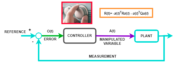
- Q-function (\(Q(s, a)\)) is somewhat analogous to the stage cost \(\ell(x_t, u_t)\) in MPC.
- \(Q(s, a)\) represents the immediate reward for taking action \(a\) in state \(s\), plus the expected future cumulative reward.
- In MPC, the cost function includes a stage cost (immediate penalty) and a terminal cost.
- Value function (\(V(s)\)) is analogous to the terminal cost \(\phi(x_T)\) in MPC.
- \(V(s)\) represents the cost-to-go from state \(s\).
- In MPC, the terminal cost function ensures stability and optimal performance beyond the finite horizon.
Q-Learnig
Q-Learning is a model-free, off-policy reinforcement learning algorithm that learns an optimal action-selection policy by iteratively updating Q-values. It is based on the Bellman equation and uses the Temporal Difference (TD) learning method to estimate future rewards. The Q-value update rule is:
\[Q(s, a) \leftarrow Q(s, a) + \alpha \left[ r + \gamma \max_{a'} Q(s', a') - Q(s, a) \right]\]where \(\alpha\) is the learning rate, \(r\) is the reward, and \(\gamma\) is the discount factor. A key challenge in Q-learning is the exploration-exploitation trade-off, which is often handled using ε-greedy exploration, where the agent selects a random action with probability ε and the best-known action otherwise.
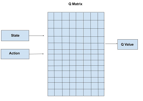
Q-learning converges to the optimal policy given sufficient exploration but struggles with large state spaces due to the need for a table storing all Q-values. Deep Q-Learning (DQN) addresses this limitation by approximating Q-values with a neural network.
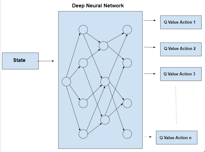
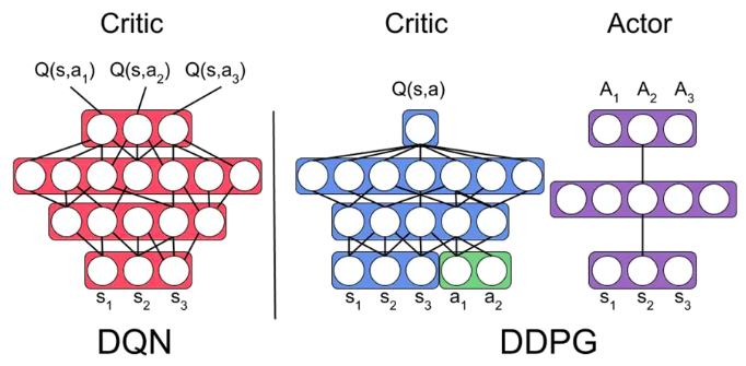
Deep Q-Learnig
Deep Q-Learning (DQN) improves upon traditional Q-Learning by using a deep neural network to approximate the Q-value function, making it scalable to high-dimensional state spaces where tabular Q-learning is infeasible. DQN introduces the experience replay buffer to improve learning stability. The replay buffer stores past experiences (state, action, reward, next state) and allows the agent to sample mini-batches for training, instead of learning from consecutive transitions. This breaks temporal correlations, improves sample efficiency, and reduces overfitting to recent experiences. Target network is also used to stabilize training by maintaining a lagged version of the Q-network to reduce oscillations.
While DQN enables learning complex policies in discrete action spaces, it struggles with continuous action spaces, requiring adaptations like DDPG. Additionally, DQN is sample inefficient, requiring large amounts of data to generalize well, and suffers from overestimation bias in Q-values. Despite these limitations, DQN has been successfully applied to discrete control tasks, and the later section of this blog post details the use of DQN for solving cartpole balancing task in Isaac Gym simulator, with discrete action space [-1, 0, 1] (*self.max_push_effort).
Target Network & Soft Update
A target network is used in reinforcement learning (RL) algorithms like DQN and DDPG to stabilize training by maintaining a lagged version of the main network for Q-value estimation. The soft update method gradually updates the target network with a weighted mix of itself and the main network using a factor \(\tau\), preventing drastic changes that cause instability. This reduces overestimation bias and smooths learning, avoiding divergence. Below is the implementation of soft update function used in DQN (and DDPG) for Isaac Gym cartpole environment. \(\tau\) is chosen to be 0.995.
def soft_update(net, net_target, tau):
    for param_target, param in zip(net_target.parameters(), net.parameters()):
        param_target.data.copy_(param_target.data * tau + param.data * (1.0 - tau))
In PyTorch, .parameters() returns an iterable of all learnable parameters (weights and biases) in a neural network, allowing updates during training. The .data attribute provides direct access to tensor values without tracking gradients, enabling manual updates like soft updates for target networks.
Implementation Details (dqn.py)
DQN updates its parameters using TD loss and a soft update for the target network. The update process follows these steps:
- Sample a mini-batch of transitions \((s, a, r, s')\) from the replay buffer.
Compute the target Q-value using the target network:
\[y = r + \gamma \max_{a'} Q_{\text{target}}(s', a')\]where \(\gamma\) is the discount factor.
Compute the current Q-value from the main network:
\[Q(s, a)\]Calculate the TD loss using Mean Squared Error (MSE) or using L1 loss in this case:
\[L = (y - Q(s, a))^2\]- Backpropagate the loss to update the q network’s parameters using gradient descent.
Soft update the target network:
\[\theta' \leftarrow \tau \theta' + (1 - \tau) \theta\]ensuring smooth updates for stability.
This procedure helps reduce overestimation bias and training instability, leading to more reliable learning in discrete action spaces. Implementation for DQN in Isaac Gym cartpole environment is shown as follows.
    def update(self, replay_buffer):
        # policy update using TD loss
        self.optimizer.zero_grad()

        obs, act, reward, next_obs, done_mask = replay_buffer.sample(self.mini_batch_size)
        q_table = self.q(obs)

        act_idx = act + 1 # maps back to the prediction space (0,1,2) for indexing
        q_val = q_table[torch.arange(self.batch_size), act_idx.long()]

        # Get optimal q value at next time step using target network
        with torch.no_grad():
            q_table_next = self.q_target(next_obs)
            idx_optimal = torch.argmax(q_table_next, dim=1)
            q_val_next = q_table_next[torch.arange(q_table_next.size(0)),idx_optimal]

        # If it is done, then no future reward
        target = reward + self.discount * q_val_next * done_mask
        self.loss = F.smooth_l1_loss(q_val, target)

        self.loss.backward()
        self.optimizer.step()

        # soft update target networks
        soft_update(self.q, self.q_target, self.tau)
        self.score += torch.mean(reward.float()).item() / self.num_eval_freq
Deep Deterministic Policy Gradient (DDPG)
Deep Deterministic Policy Gradient (DDPG) is an off-policy reinforcement learning algorithm designed for continuous action spaces, unlike DQN, which is limited to discrete actions. DDPG extends DQN by incorporating the actor-critic framework, where the actor learns a deterministic policy, and the critic estimates Q-values. It combines DQN’s target network and experience replay with policy gradients, enabling stable learning in high-dimensional continuous spaces. Additionally, DDPG avoids ε-greedy exploration by using Ornstein-Uhlenbeck noise for smoother exploration. This makes DDPG a natural extension of DQN, adapting it to complex robotic control tasks where discrete actions are insufficient.
Actor Critic Method
The actor-critic method is a hybrid approach that combines value-based and policy-based learning. The critic estimates the value function (e.g., Q-values), while the actor updates the policy based on the critic’s feedback. This reduces variance compared to pure policy-based methods and speeds up learning. In DDPG, the critic learns using the Bellman equation, similar to DQN, while the actor optimizes policy gradients to directly adjust actions. This dual-network structure allows DDPG to handle continuous control problems efficiently, balancing stability (via the critic) and exploration (via the actor).
Deterministic Policy & Action Noise
The “deterministic” in Deep Deterministic Policy Gradient (DDPG) refers to the fact that the actor network outputs a single, fixed action for a given state rather than a probability distribution over actions. In contrast, stochastic policy-based methods like PPO output a probability distribution, allowing for action sampling, which is beneficial for exploration. DDPG’s deterministic policy is represented as:
\[a = \pi(s|\theta^\pi)\]where \(\pi\) is the actor network, which directly mapping state \(s\) to action \(a\). This deterministic approach improves sample efficiency but requires explicit exploration mechanisms.
Since DDPG’s policy is deterministic, it lacks inherent exploration, which can lead to poor performance in complex environments. To encourage exploration, action noise is added to the selected action during training:
\[a' = \pi(s|\theta^\pi) + \mathcal{N}\]where (\mathcal{N}) is a noise function, commonly Ornstein-Uhlenbeck (OU) noise for temporally correlated exploration or Gaussian noise. This noise helps DDPG explore better by preventing it from getting stuck in local optima.
Implementation Details (ddpg.py)
Similar to DQN, DDPG also uses the target, for both actor and critic networks. Thus, total of four neural networks need to be initialized at the beginning. Critic Network is updated by doing gradient descent to minimize the TD Loss, and Actor Netowrk is updated by doing gradient ascent to maximize the reward (Q-value). Picture below illustrate the procedures for DDPG algorithm.
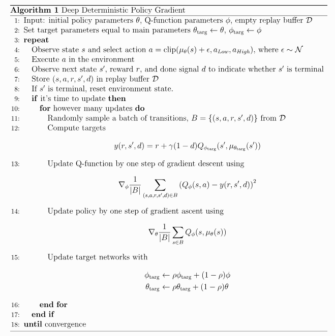
In the context of cartpole environment, the continous action space is constrained to [-1, 1] (*self.max_push_effort), thus, tanh activation function is used for the output of actor networks. Function for updating parameters of DDPG’s neural networks are shown below.
    def update(self, replay_buffer):
        # Sample a batch of experience from the replay buffer
        with torch.no_grad():
            obs, act, reward, next_obs, done_mask = replay_buffer.sample(self.mini_batch_size)
            next_action = self.actor_target.forward(next_obs)
            q_val_next = self.critic_target.forward(next_obs, next_action)
            reward = reward.unsqueeze(1)
            done_mask = done_mask.unsqueeze(1)
            target = reward + self.discount * q_val_next * done_mask

        q_val = self.critic.forward(obs, act)
        self.critic_loss = F.mse_loss(q_val, target)

        self.critic_optimizer.zero_grad()
        # critic_loss.backward(retain_graph=True)
        self.critic_loss.backward()
        self.critic_optimizer.step()

        # Actor update (maximize Q-value)
        mu = self.actor.forward(obs)
        self.actor_loss = -self.critic.forward(obs, mu).mean()  # negative because we want to maximize Q
        self.actor_optimizer.zero_grad()
        self.actor_loss.backward()
        self.actor_optimizer.step()

        # Update the target networks (using soft update)
        soft_update(self.critic, self.critic_target, self.tau)
        soft_update(self.actor, self.actor_target, self.tau)

        self.reward += torch.mean(reward.float()).item() / self.num_eval_freq
Summary
- Reinforcement Learning (RL) provides a framework for sequential decision-making, where an agent learns optimal policies through interaction with an environment. Concepts like policy iteration and value iteration help in understanding policy updates, drawing analogies with Model Predictive Control (MPC) in optimal control.
- Q-Learning is a fundamental off-policy, model-free RL algorithm that updates Q-values using the Bellman equation, balancing the exploration-exploitation trade-off through techniques like ε-greedy exploration.
- Deep Q-Learning (DQN) extends Q-learning by approximating Q-values with neural networks, using techniques such as experience replay and target networks to improve stability and efficiency.
- Deep Deterministic Policy Gradient (DDPG) further advances RL for continuous action spaces by combining DQN’s value-based learning with actor-critic policy updates, utilizing a deterministic policy and action noise for exploration.
References
- Deep Deterministic Policy Gradient (OpenAI Spinning Up)
- L21: Temporal Difference Learning
- Q-Learning Explained - A Reinforcement Learning Technique & Deep Q-Learning - Combining Neural Networks and Reinforcement Learning (Deep Lizard RL Series)
- Reinforcement Learning - “DDPG” explained and M16V06 Deep deterministic policy gradient
- minimal-isaac-gym, DPG-Pytorch, cartpole-dqn-ddpg-ppo
- How DDPG (Deep Deterministic Policy Gradient) Algorithms works in reinforcement learning ?