Implementation Details of TD3-SAC-Gymnasium

Twin Delayed Deep Deterministic Policy Gradient (TD3) and Soft Actor-Critic (SAC) are off-policy actor-critic algorithms designed for continuous control tasks where classic DDPG can be unhandy. TD3 stabilizes learning with tricks such as double Q-networks, delayed policy updates, and target policy smoothing to reduce overestimation bias. SAC instead learns a stochastic policy by maximizing both task reward and entropy, encouraging robust and exploratory behaviors. This blog post explains core components and implementation details of both algorithms. Corresponding PyTorch implementation can be found at this repository.

Categories of RL Algorithms

Before diving into TD3 and SAC, it is helpful to place them within the broader landscape of reinforcement learning (RL). In this section we briefly review two common ways of categorizing RL algorithms: (i) how they represent and optimize behavior (value-based, policy-based, or actor–critic), and (ii) how they use experience (on-policy vs off-policy). This perspective will make it clearer why TD3 and SAC are usually described as off-policy actor–critic algorithms for continuous control.

• Value-based vs Policy-based vs Actor–Critic

  • Value-based methods.
    Value-based algorithms learn a value function, such as a state–action value \(Q(s,a)\) or state value \(V(s)\), and derive a policy by acting greedily with respect to this estimate. For example, a greedy policy is

    \[\pi(s) = \arg\max_a Q(s,a).\]

    Classic examples include tabular Q-learning and deep Q-networks (DQN). The policy is implicit in the value function; there is usually no separate set of policy parameters.

  • Policy-based methods (pure policy gradient).
    Pure policy-gradient methods parameterize the policy directly as \(\pi_\theta(a \mid s)\) and optimize the expected return

    \[J(\theta) = \mathbb{E}_{\pi_\theta}\!\left[\sum_{t=0}^{\infty} \gamma^t r_t \right]\]

    via gradients of the form

    \[\nabla_\theta J(\theta) = \mathbb{E}_{\pi_\theta}\!\big[ \nabla_\theta \log \pi_\theta(a_t \mid s_t)\, \hat{G}_t \big],\]

    where \(\hat{G}_t\) is some return estimate. The simplest example is REINFORCE, which can work without a learned value function by using Monte Carlo returns as \(\hat{G}_t\).

  • Actor–critic methods (policy gradient with a critic).
    Actor–critic algorithms combine both ideas. An actor \(\pi_\theta(a \mid s)\) chooses actions, while a critic estimates a value function (e.g., \(V_\phi(s)\), \(Q_\phi(s,a)\), or an advantage \(A_\phi(s,a)\)) to provide low-variance learning signals for the actor:

    \[\nabla_\theta J(\theta) \approx \mathbb{E}\!\big[ \nabla_\theta \log \pi_\theta(a_t \mid s_t)\, \hat{A}_\phi(s_t,a_t) \big].\]

    Algorithms such as A2C/A3C, TRPO (in its common actor–critic form), PPO, TD3, and SAC fall into this category: they use a policy-gradient objective together with an explicit value function learned by the critic.

• On-policy vs Off-policy

  To explain this distinction, it is useful to separate two roles a policy can play:

  • Behavior policy \(\mu(a \mid s)\): the policy that actually acts in the environment to generate data \((s_t, a_t, r_t, s_{t+1})\).

  • Target policy \(\pi(a \mid s)\): the policy we are trying to evaluate or improve in our update rule.

  • On-policy algorithms
    On-policy methods learn about a target policy using data collected from (essentially) the same policy: \(\mu(a \mid s) \approx \pi(a \mid s).\) In practice, the behavior policy might add a bit of exploration noise, or we might update \(\pi\) slightly during training, but the algorithm is designed so that the data always come from a policy very close to the one being optimized .
    Examples:
    • SARSA learns the value of the current \(\epsilon\)-greedy policy.
    • PPO collects rollouts with an old policy \(\pi_{\text{old}}\) and then updates \(\pi_\theta\) while constraining it (via clipping or a KL penalty) so that \(\pi_\theta \approx \pi_{\text{old}}\). Old data are only used for a few epochs and then discarded.
  • Off-policy algorithms
    Off-policy methods allow the behavior and target policies to be different: \(\mu(a \mid s) \neq \pi(a \mid s).\) This makes it possible to reuse past experience, learn from old versions of the policy, or even learn from demonstrations generated by some other agent .
    Examples:
    • Q-learning and DQN typically use an \(\epsilon\)-greedy behavior policy \(\mu\), but update towards the greedy policy \(\pi_{\text{greedy}}(s) = \arg\max_a Q(s,a),\) so \(\mu \neq \pi_{\text{greedy}}\).
    • DDPG, TD3, and SAC store transitions in a replay buffer and train the current actor–critic using data that were collected many steps ago under different (more exploratory) policies. This clear separation between data collection and policy improvement is what makes them off-policy.

In the following sections we will see that TD3 and SAC sit in the intersection of these categories: they are off-policy actor–critic algorithms that learn a critic \(Q_\phi(s,a)\) and a continuous-control actor \(\pi_\theta(a \mid s)\) using replayed experience.

Twin Delayed Deep Deterministic Policy Gradient (TD3)

Twin Delayed Deep Deterministic Policy Gradient (TD3) is a widely used algorithm for continuous-control RL that builds directly on Deep Deterministic Policy Gradient (DDPG). Like DDPG, TD3 uses an actor–critic architecture with a deterministic policy (actor) and a Q-function approximator (critic), trained off-policy using a replay buffer and target networks.

In practice, however, DDPG is notoriously brittle: small hyperparameter changes often cause the critic’s Q-values to explode and the learned policy to collapse. TD3 preserves the overall structure, but adds several targeted modifications—most notably clipped double Q-learning, delayed policy updates, and target policy smoothing—to systematically reduce value overestimation and stabilize critic learning across a wide range of tasks.

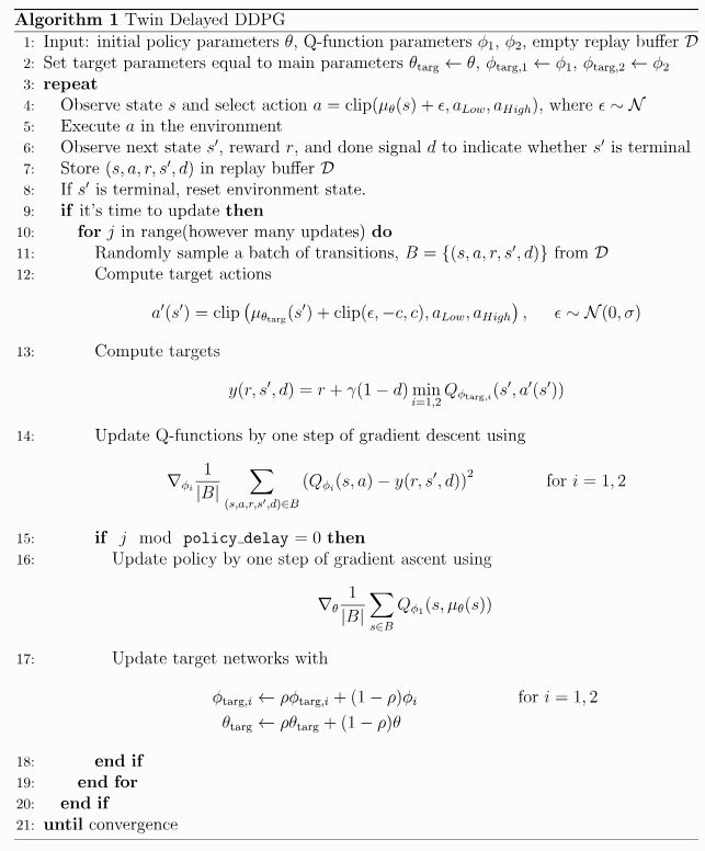
One of the most frequently mentioned issues with RL training in TD3 paper is about Q-value overestimation and critic divergence. Let’s dive deeper into this critical part and followed by the critic network update implementation of TD3.

• Overestimation and critic divergence

  • Overestimation bias.
    With a single critic and an actor trained to maximize \(Q\), the policy tends to pick actions where the critic’s random errors are positive, leading to systematically over-optimistic value estimates.

  • Bias compounding via bootstrapping.
    Targets use \(y = r + \gamma Q(s', \pi(s')).\) If \(Q\) is already overestimated, each TD update pushes it even higher, and the actor further exploits these inflated regions.

  • Critic divergence.
    Combined with function approximation and off-policy data (the “deadly triad”), these biased, self-referential targets can make Q-values and TD errors grow without bound instead of converging.

  • Practical effect.
    Diverging critics produce meaningless gradients, exploding losses, and unstable or collapsed policies. TD3’s core tricks explicitly tackle this loop, making the critic more conservative and its updates more stable.

def update_critic(self, obs, action, reward, next_obs, 
                  terminated_flag, logger, step):
    # Calculate the target Q value
    with torch.no_grad():
        # ! start below
        # Select action according to policy and add clipped noise
        noise = (torch.randn_like(action) * self.policy_noise).clamp(-self.noise_clip, self.noise_clip)	
        next_action = (self.actor_target(next_obs) + noise).clamp(self.min_action, self.max_action)

        # Compute the target Q value
        target_Q1, target_Q2 = self.critic_target(next_obs, next_action)
        target_Q = torch.min(target_Q1, target_Q2)
        target_Q = reward + (1-terminated_flag) * self.discount * target_Q

    # get current Q estimates
    current_Q1, current_Q2 = self.critic(obs, action)
    critic_loss = F.mse_loss(current_Q1, target_Q) +\
          F.mse_loss(current_Q2, target_Q)
    logger.log('train_critic/loss', critic_loss, step)

    # Optimzer the critic
    self.critic_optimizer.zero_grad()
    critic_loss.backward()
    self.critic_optimizer.step()

For the actor update, it is worth noting that there are two types of noises used in the TD3 algorithm, both are explained in more detail as below. In addition, when interacting with the environment, you don’t want gradients for that actor network forward pass. You’re just choosing an action, not updating the network from it.

Thus, we only update the networks from replayed batches. Wrapping agent.get_action() in torch.no_grad() avoids building computation graphs for these forward passes, saving memory and time and preventing accidental backprop through action sampling. Always enable grads only inside the update step.

• Policy noise vs exploration noise
  • Exploration noise (interaction with the environment)
    • Added to the action sent to the environment during data collection.

    • Example:

      \[a_{\text{env}} = \pi_\theta(s) + \epsilon, \qquad \epsilon \sim \mathcal{N}(0, \sigma_{\text{expl}}^{2}).\]
    • Purpose: encourage state–action space exploration so the replay buffer contains diverse trajectories.
    • Affects the behavior policy only; it does not change the TD target formula.
  • Policy noise (target policy smoothing in TD3)
    • Added inside the critic update to the target policy’s action when computing the TD target.

    • Example:

      \[\tilde{a}' = \pi_{\bar\theta}(s') + \eta, \qquad \eta \sim \mathcal{N}(0, \sigma_{\text{policy}}^{2}), \quad \eta \text{ clipped}\] \[y = r + \gamma \min_i Q_{\bar\phi_i}(s', \tilde{a}').\]
    • Purpose: smooth the target Q-function and reduce overestimation by learning a value for a local neighborhood around the policy action instead of a single sharp point.
    • Affects only training of the critic (and indirectly the actor); never used for actual actions in the environment.

def update_actor(self, obs, logger, step):
    action = self.actor(obs)
    actor_Q1, actor_Q2 = self.critic(obs, action)

    # !only select Q1 based on the algorithm
    actor_loss = -actor_Q1.mean()

    logger.log('train_actor/loss', actor_loss, step)

    self.actor_optimizer.zero_grad()
    actor_loss.backward()
    self.actor_optimizer.step()

def update(self, replay_buffer, logger, step):
    obs, action, reward, next_obs, terminated_flag = replay_buffer.sample(self.batch_size)
    logger.log('train/batch_reward', reward.mean(), step)
    self.update_critic(obs, action, reward, 
                        next_obs, terminated_flag, logger, step)

    if step % self.policy_update_frequency == 0:
        self.update_actor(obs, logger, step)

        # update both target actor and target critic networks
        utils.soft_update_params(self.critic, self.critic_target, self.tau)
        utils.soft_update_params(self.actor, self.actor_target, self.tau)

• TD3 Results

Stochastic Policy

In stochastic policies, the agent samples actions from a state-conditioned distribution \(\pi_\theta(\cdot\mid s)\) to enable exploration and define a valid density for entropy regularization. Soft Actor-Critic (SAC) is a stochastic, entropy-regularized actor–critic that maximizes value while encouraging high-entropy behavior. Practically, SAC samples from an unbounded Gaussian and applies a smooth \(\tanh\) squashing to satisfy action bounds; the change-of-variables rule yields a correct log-probability, so both gradients and entropy are well defined. Let’s now get into details of these operations.

• Gradient Estimators

  We seek gradients of an expectation where the sampled action depends on parameters \(\theta\):

  \[\nabla_\theta\,\mathbb{E}_{a\sim \pi_\theta(\cdot\mid s)}\!\big[L(s,a)\big].\]

  1. Score-function (REINFORCE):

  \[\nabla_\theta\,\mathbb{E}_{a\sim \pi_\theta}\!\big[L(s,a)\big] = \mathbb{E}_{a\sim \pi_\theta}\!\big[L(s,a)\,\nabla_\theta \log \pi_\theta(a\mid s)\big].\]

  This works for any distribution, but often high variance.

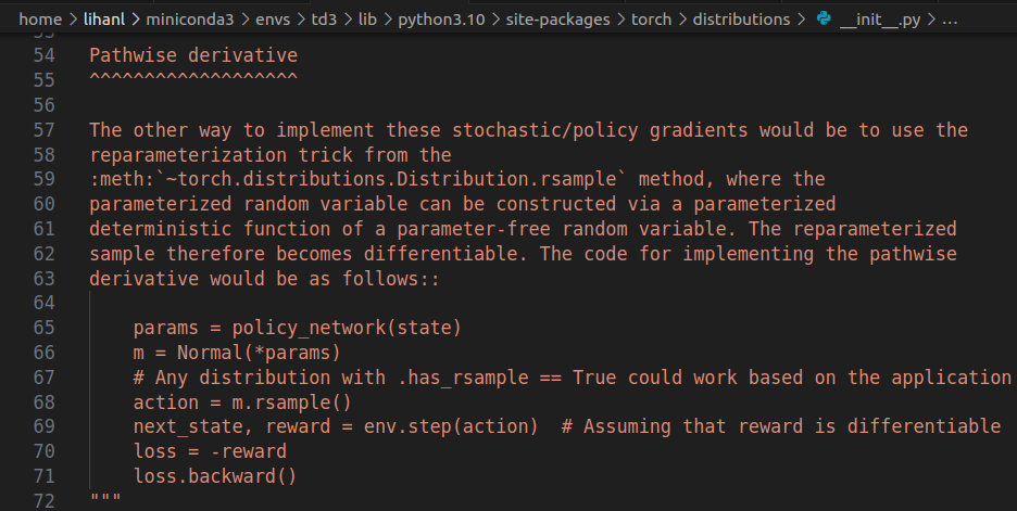
  2. Pathwise derivative (reparameterization):

  If we can write \(a = g_\theta(\varepsilon, s)\) with \(\varepsilon \sim p(\varepsilon)\) independent of \(\theta\), then

  \[\nabla_\theta \,\mathbb{E}_{\varepsilon}\!\big[\,L\!\big(s, g_\theta(\varepsilon, s)\big)\,\big] \;=\; \mathbb{E}_{\varepsilon}\!\big[\,\nabla_\theta L\!\big(s, g_\theta(\varepsilon, s)\big)\,\big].\]

  Autodiff can then backprop through the deterministic map \(g_\theta\), yielding much lower variance than score-function gradients.

  In SAC with tanh-squashed Gaussians:

  \[\varepsilon \sim \mathcal{N}(0, I),\qquad z = \mu_\theta(s) + \sigma_\theta(s)\odot \varepsilon,\qquad a = \tanh(z).\]

  So \(a = g_\theta(\varepsilon, s)\). We use the pathwise gradient for both the \(Q(s,a)\) term and the entropy term \(\alpha \log \pi(a\mid s)\) (the latter is well-defined thanks to the change-of-variables + Jacobian). Picture below shows the explanation from PyTorch.

• Tanh Normalization

  1. Quick clarifications

  • log_prob (aka \(\log p_X(x)\)) is a number for a particular sample \(x\).

  • Entropy \(H(X)\) is not \(-\log p_X(x)\) at some \(x\). It is the expectation of \(-\log p_X(X)\) over the random variable \(X\):

  \[\boxed{\,H(X)\;=\;-\;\mathbb{E}_{X}\!\left[\log p_X(X)\right]\,}.\]

  • Change-of-variables (per sample): Let \(Y=f(X)\) be a bijection with Jacobian \(J_f(x)=\tfrac{\partial y}{\partial x}\). The identity below is used for SAC to calculate each sampled action, and it is also what dist.log_prob() returns (per-sample log-probability).

    \[\boxed{\,\log p_Y(y)\;=\;\log p_X(x)\;-\;\log\!\big|\det J_f(x)\big|\,,\qquad x=f^{-1}(y)\,}.\]

    The Jacobian of the transformation \(a = \tanh(z)\) is diagonal with entries \(1 - \tanh^2(z),\) so the log-determinant of the Jacobian is

    \[\log \left| \det J \right| = \sum_i \log\!\left(1 - \tanh^2(z_i)\right).\]

    Based on this implementation from tensorflow, we used a more numerically stable equivalent expression:

    \[\log\!\left(1 - \tanh(x)^2\right) = 2 \,\big( \log 2 - x - \mathrm{softplus}(-2x) \big).\]

    Both forms are mathematically identical. The stable form prevents catastrophic cancellation when \(|x|\) is large (where \(\tanh(x) \approx \pm 1\) and \(1 - \tanh(x)^2\) underflows). The code block below shows the definition of example imports and class definition to realize the calculation mentioned above.

  import torch, math
  from torch.distributions import MultivariateNormal, TransformedDistribution, constraints
  from torch.distributions.transforms import Transform
  
  class Tanh2D(Transform):
      # Define the transformation properties
      domain = constraints.real_vector
      codomain = constraints.interval(-1.0, 1.0)
      bijective = True
      sign = +1
      def __init__(self): super().__init__(cache_size=1)
      def _call(self, x):  return x.tanh()
      def _inverse(self, y): return 0.5 * (y.log1p() - (-y).log1p())
      def log_abs_det_jacobian(self, x, y):
          ladj_elem = 2.0 * (math.log(2.0) - x - torch.nn.functional.softplus(-2.0 * x))
          return ladj_elem.sum(dim=-1)
  
  m = torch.tensor([0.5, -0.8])
  Sigma = torch.tensor([[1.4, 0.3],[0.3, 1.1]])
  X = MultivariateNormal(m, Sigma)
  Y = TransformedDistribution(X, [Tanh2D()])
  

  2. Entropy under a transform (an expectation)

  Start from the definition

  \[H(Y)\;=\;-\;\mathbb{E}_{Y}\!\left[\log p_Y(Y)\right].\]

  Change variables \(Y=f(X)\), then plug the per-sample formula:

  \[\begin{aligned} H(Y) &= -\,\mathbb{E}_{X}\!\left[\log p_Y\!\big(f(X)\big)\right] \\ &= -\,\mathbb{E}_{X}\!\left[\log p_X(X) - \log\!\big|\det J_f(X)\big|\right] \\ &= \underbrace{-\,\mathbb{E}_{X}\!\left[\log p_X(X)\right]}_{H(X)} \;+\;\mathbb{E}_{X}\!\left[\log\!\big|\det J_f(X)\big|\right]. \end{aligned}\]

  So

  \[\boxed{\,H(Y)\;=\;H(X)\;+\;\mathbb{E}_{X}\!\left[\log\!\big|\det J_f(X)\big|\right]\,}.\]

  Yes. In SAC the entropy term is the conditional entropy of the policy:

  \[\mathbb{E}_{s \sim \mathcal{D},\, a \sim \pi(\cdot \mid s)} \left[ - \log \pi(a \mid s) \right].\]

  In code, for a minibatch of states obs (size 1024) you draw actions with action = dist.rsample(), then compute log_prob = dist.log_prob(action). Averaging -log_prob over the batch is exactly a Monte-Carlo estimate of the expectation above (expectation over both the replay distribution of states and the policy’s action distribution conditioned on each state). That’s why people often log it as “entropy”.

  • In the actor loss, you don’t put the minus—SAC uses

    \[\alpha \log \pi(a \mid s) - Q(s,a).\]

  • For metrics, people often report the following for readability.

    \[\text{entropy} = -\,\text{log_prob.mean()}\]

xs = torch.tensor([[ 0.0,  0.0],
                   [ 1.2, -0.7],
                   [-1.5,  2.0]], dtype=torch.get_default_dtype())
ys = xs.tanh()
logpX = X.log_prob(xs)
logpY = Y.log_prob(ys)
logabsdet_dYdX = (2.0 * (math.log(2.0) - xs - torch.nn.functional.softplus(-2.0 * xs))).sum(dim=-1)
rhs = logpX - logabsdet_dYdX

print("=== 2D tanh transform: log-prob identity (3 points) ===")
for i in range(xs.size(0)):
    print(f"x={xs[i].tolist()}, y={ys[i].tolist()}")
    print(f"  log p_Y(y)                   = {logpY[i].item():.6f}")
    print(f"  log p_X(x) - log|det(dY/dX)| = {rhs[i].item():.6f}")
    print(f"  residual                     = {(logpY[i]-rhs[i]).item():.3e}")
    print()

HX = X.entropy().item()
N = 200_000
with torch.no_grad():
    x_samp = X.rsample((N,))
    ladj_elem = 2.0 * (math.log(2.0) - x_samp - torch.nn.functional.softplus(-2.0 * x_samp))
    E_logdetJ = ladj_elem.sum(dim=-1).mean().item()
    y_samp = torch.tanh(x_samp)
    HY_mc = -(Y.log_prob(y_samp)).mean().item()

HY_expected = HX + E_logdetJ
print("=== Entropy check for Y = tanh(X) in R^2 ===")
print(f"H(X) analytic                     = {HX:.6f}")
print(f"E_X[ log|det(dY/dX)| ] (MC)       = {E_logdetJ:.6f}")
print(f"H(Y) expected via identity        = {HY_expected:.6f}")
print(f"H(Y) Monte Carlo via samples      = {HY_mc:.6f}")

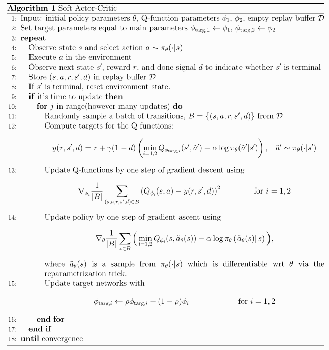
Soft Actor-Critic (SAC)

After the introduction of several key concepts mentioned previously, let’s break SAC down into pieces for more detailed explanation.

• Critic Updates

  Besides the use of target network, which is similar to DDGP, in SAC critic network update, there are several implementation details that may need to dwell on. We now go over each of them individually and attach the PyTorch implementation snippet at the end of this section.

  1) self.alpha.detach() for temperature

  In the critic update we want to update only the critic parameters \(\phi\) by minimizing the MSE between the current Q-values and a target:

  \[\mathcal{L}_{\text{critic}}(\phi) = \mathbb{E} \Bigg[ \sum_{i=1}^{2} \big( Q_{\phi}^{(i)}(s,a) - y \big)^2 \Bigg],\]

  where the target is

  \[y = r + \gamma (1-d) \underbrace{ \Big( \min_{j} Q_{\bar\phi}^{(j)}(s', a') - \alpha \log \pi_{\theta}(a' \mid s') \Big) }_{\text{soft value target}}.\]
  • \(\alpha\) (the temperature) is a separate parameter (trained by a separate loss) that should not receive gradients from the critic loss.
  • If you leave \(\alpha\) attached, then \(\nabla_{\alpha}\mathcal{L}_{\text{critic}}\) will be non-zero and the critic step will (incorrectly) push \(\alpha\).
  • self.alpha.detach() zeroes that gradient path so the critic update only modifies \(\phi\).

  You will see the same idea in the actor update: we often detach \(\alpha\) to avoid cross-talk from the actor loss into the temperature learner .

  2) Meaning of target_V

  target_V is a single-sample Monte Carlo estimate of the soft value \(V(s')\):

  \[\hat{V}(s') = \min_{j} Q_{\bar\phi}^{(j)}(s', a') - \alpha \log \pi_{\theta}(a' \mid s').\]

  The expectation over \(a' \sim \pi(\cdot \mid s')\) is approximated with one action sample (rsample()), which is standard and unbiased (with variance reduced by large batch sizes).

  • target_Q is the one-step bootstrap target \(y\) for the critic MSE: reward plus discounted target_V, masked by \((1 - \text{terminated_flag})\).
  • The double Q term (\(\min\) of two target critics) reduces positive bias / overestimation.

  Thus, this way of calculation uses a single action sample per next state to approximate the expectation inside \(V(s')\).

  3) Use of with torch.no_grad() when computing targets

  When building the bootstrapped target \(y\), you do not want gradients to flow into:

  • the target critic (frozen parameters \(\bar\phi\)),
  • the actor (when sampling \(a'\) for the critic target),
  • or the log_prob term.

  Using with torch.no_grad() around the target computation ensures these components are treated as constants for the purpose of the critic update.

def update_critic(self, obs, action, reward, next_obs, 
                      terminated_flag, logger, step):
    # Calculate the target Q value
    with torch.no_grad():
        dist = self.actor(next_obs)
        next_action = dist.rsample()
        log_prob = dist.log_prob(next_action).sum(-1, keepdim=True)
        target_Q1, target_Q2 = self.critic_target(next_obs, next_action)
        # !.detach() is important here
        target_V = torch.min(target_Q1, target_Q2) - self.alpha.detach() * log_prob

        target_Q = reward + (1 - terminated_flag) * self.discount * target_V
        target_Q = target_Q.detach()

    # get current Q estimates
    current_Q1, current_Q2 = self.critic(obs, action)
    critic_loss = F.mse_loss(current_Q1, target_Q) +\
          F.mse_loss(current_Q2, target_Q)
    logger.log('train_critic/loss', critic_loss, step)

    # Optimzer the critic
    self.critic_optimizer.zero_grad()
    critic_loss.backward()
    self.critic_optimizer.step()

• Actor and Temperature Updates

  1. Temperature loss design and gradient intuition

  Many implementations optimize log_alpha with the loss

  \[\mathcal{L}(\log \alpha) = \mathbb{E} \Big[ \alpha \big( - \log \pi(a \mid s) - \mathcal{H}_{\text{tgt}} \big) \Big],\]

  where the term \(\big( - \log \pi(a \mid s) - \mathcal{H}_{\text{tgt}} \big)\) is detached in code.

  Taking the derivative w.r.t. \(\log \alpha\) (using \(\alpha = e^{\log \alpha}\)):

  \[\nabla_{\log \alpha} \mathcal{L} = \alpha \, \mathbb{E} \big[ - \log \pi(a \mid s) - \mathcal{H}_{\text{tgt}} \big].\]

  This needs double-check!

  • If the current entropy is too low: \(H(\pi) = \mathbb{E}[- \log \pi] < \mathcal{H}_{\text{tgt}} \Rightarrow \text{bracket} < 0 \Rightarrow \text{gradient} < 0 \Rightarrow\) gradient descent increases \(\log \alpha \Rightarrow \alpha\) goes up \(\Rightarrow\) the actor puts more weight on entropy \(\Rightarrow\) entropy rises.

  • If the current entropy is too high: \(H(\pi) > \mathcal{H}_{\text{tgt}} \Rightarrow \text{bracket} > 0 \Rightarrow \text{gradient} > 0 \Rightarrow\) gradient descent decreases \(\log \alpha \Rightarrow \alpha\) goes down \(\Rightarrow\) the entropy weight weakens \(\Rightarrow\) entropy falls.

  This yields an automatic temperature that tracks the desired entropy level.

  2. Use of .detach()

  tensor.detach() returns a view of the tensor with the same values but no gradient history. During backprop, gradients do not flow through a detached tensor. It is a stop-grad operation. The temperature \(\alpha\) is trained to make the actual policy entropy match a target entropy \(\mathcal{H}_{\text{tgt}}\).

  • We optimize only \(\alpha\) (often its log-parameter log_alpha), keeping the actor fixed during this step.
  • If we did not detach \((- \text{log_prob} - \text{target_entropy})\), gradients from the \(\alpha\) update would also flow back into the actor, entangling updates and destabilizing learning.
  • By calling .detach(), the entropy measurement is treated as a constant sample when updating \(\alpha\). Gradients flow only to \(\alpha\).

  (You see the same pattern in the actor loss: actor_loss = alpha.detach() * log_prob - Q.
  There we stop-grad through \(\alpha\) so the actor step does not update \(\alpha\).)

  3. -log_prob.mean() for entropy

  For a batch of \(1024\) states \(s_i\) and one action sample \(a_i \sim \pi(\cdot \mid s_i)\) per state:

  \[-\frac{1}{1024} \sum_{i=1}^{1024} \log \pi(a_i \mid s_i) \;\approx\; \mathbb{E}_{s \sim \mathcal{D}} \Big[ \mathbb{E}_{a \sim \pi(\cdot \mid s)} \big[ - \log \pi(a \mid s) \big] \Big],\]

  which is exactly a Monte-Carlo estimate of the policy entropy averaged over the replay-state distribution. (And dist.log_prob(action) already includes the tanh + scaling Jacobians, so it is the true bounded-policy log-prob.)

  Shape-wise:

  • dist.log_prob(action) → \([ \text{batch}, \text{action_dim} ]\) (factorized)
  • .sum(-1, keepdim=True) → \([ \text{batch}, 1 ]\) gives per-sample \(\log \pi(a \mid s)\)
  • .mean() over batch → scalar estimate of \(\mathbb{E}[ \log \pi(a \mid s) ]\)
    (and \(-\text{mean}\) is the entropy estimate)

  def update_actor_and_alpha(self, obs, logger, step):
      dist = self.actor(obs)
      action = dist.rsample()
      log_prob = dist.log_prob(action).sum(-1, keepdim=True)
      actor_Q1, actor_Q2 = self.critic(obs, action)
  
      actor_Q = torch.min(actor_Q1, actor_Q2)
      # !.detach() is important here
      actor_loss = (self.alpha.detach() * log_prob - actor_Q).mean()
  
      logger.log('train_actor/loss', actor_loss, step)
      logger.log('train_actor/target_entropy', self.target_entropy, step)
      logger.log('train_actor/entropy', -log_prob.mean(), step)
  
      self.actor_optimizer.zero_grad()
      actor_loss.backward()
      self.actor_optimizer.step()
  
      if self.learnable_temperature:
          self.log_alpha_optimizer.zero_grad()
          # !.detach() is important here
          alpha_loss = (self.alpha * 
                        (-log_prob - self.target_entropy).detach()).mean()
          logger.log('train_alpha/loss', alpha_loss, step)
          logger.log('train_alpha/value', self.alpha, step)
          alpha_loss.backward()
          self.log_alpha_optimizer.step()
  

• SAC Results

References

1. Addressing Function Approximation Error in Actor-Critic Methodsl (TD3 Paper)
2. Soft Actor-Critic: Off-Policy Maximum Entropy Deep Reinforcement Learning with a Stochastic Actor (SAC Paper)
3. TD3, SAC (OpenAI Spinning Up)
4. Entropy Clearly Explained!!! & Intuitively Understanding the KL Divergence
5. TD3, pytorch_sac.