Shed Some Light on Proximal Policy Optimization (PPO) and Its Application

Proximal Policy Optimization (PPO) is a reinforcement learning algorithm that refines policy gradient methods like REINFORCE using importance sampling and a clipped surrogate objective to stabilize updates. PPO-Penalty explicitly penalizes KL divergence in the objective function, and PPO-Clip instead uses clipping to prevent large policy updates. In many robotics tasks, PPO is first used to train a base policy (potentially with privileged information). Then, a deployable controller is learned from this base policy using imitation learning, distillation, or other techniques. This blog explores PPO’s core principle, with code available at this repository.

Policy Gradient

Policy Gradient methods are a foundational class of algorithms in reinforcement learning (RL) that directly optimize a parameterized policy with respect to expected cumulative reward. Unlike value-based methods such as Q-learning, which aim to learn value functions and derive policies indirectly, policy gradient methods focus on learning the policy itself, often represented as a neural network that outputs a probability distribution over actions given states .

However, policy gradient methods are not without challenges—issues such as high variance in gradient estimates and sample inefficiency are well-known. To understand the core idea behind this family of methods, we begin with the most basic and historically significant example: REINFORCE, a Monte Carlo-based algorithm that illustrates how policy gradients can be estimated using sampled trajectories.

• REINFORCE

  

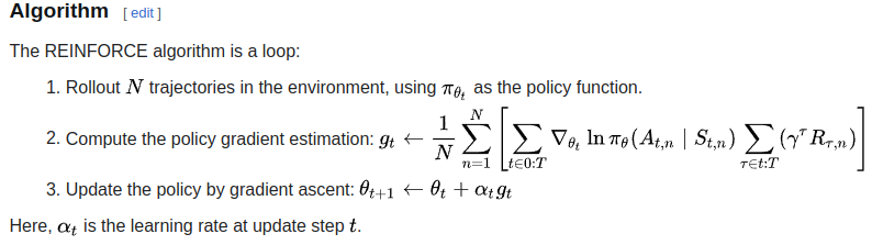
  The REINFORCE algorithm is an on-policy algorithm. By collecting \(N\) rollout trajectories, it estimates the policy gradient and optimizes the expected return of a parameterized stochastic policy. \(\pi_\theta(a \mid s)\) denotes a policy that defines a distribution over actions given a state, with parameters \(\theta\).

  In REINFORCE, the goal is to find a parameterized policy \(\pi_\theta(a \mid s)\) that maximizes expected return:

  \[\theta^* = \arg\max_\theta \mathbb{E}_{\tau \sim \pi_\theta(\tau)} \left[ \sum_t r(s_t, a_t) \right]\]

  Here, \(\tau = (s_1, a_1, s_2, a_2, \dots, s_T, a_T)\) is a trajectory sampled from the policy.

  We define the objective function as:

  \[J(\theta) = \mathbb{E}_{\tau \sim \pi_\theta(\tau)} \left[ r(\tau) \right] = \int \pi_\theta(\tau) r(\tau) \, d\tau\]

  • Derivation Using the Log Derivative Trick

    Taking the gradient of \(J(\theta)\):

    \[\nabla_\theta J(\theta) = \nabla_\theta \int \pi_\theta(\tau) r(\tau) \, d\tau = \int \nabla_\theta \pi_\theta(\tau) r(\tau) \, d\tau\]

    This is problematic because we usually cannot directly compute \(\nabla_\theta \pi_\theta(\tau)\). So we apply the log-derivative trick:

    

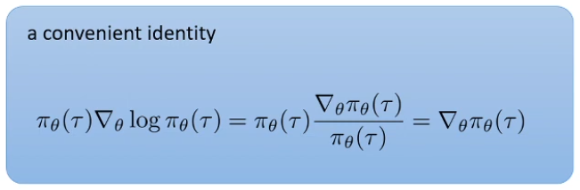
    This identity helps us convert a gradient of a probability density into something we can sample from. Substitute it in:

    \[\nabla_\theta J(\theta) = \int \pi_\theta(\tau) \nabla_\theta \log \pi_\theta(\tau) r(\tau) \, d\tau = \mathbb{E}_{\tau \sim \pi_\theta} \left[ \nabla_\theta \log \pi_\theta(\tau) r(\tau) \right]\]

  • Policy Gradient Approximation

    REINFORCE approximates this expectation using Monte Carlo samples:

    \[\nabla_\theta J(\theta) \approx \frac{1}{N} \sum_{i=1}^N \nabla_\theta \log \pi_\theta(\tau^{(i)}) R^{(i)}\]

    Where \(R^{(i)} = \sum_t r_t^{(i)}\) is the return of the \(i\)-th trajectory.

    This is a Monte Carlo policy gradient estimator.

• High Variance and the Role of the Baseline

  Despite its theoretical elegance and unbiased gradient estimates, REINFORCE suffers from high variance and delayed updates, as gradients can only be computed after full trajectory rollouts. These drawbacks motivate subsequent algorithms like Actor-Critic and Proximal Policy Optimization (PPO), which improve learning stability through value function baselines and clipped surrogate objectives.

  A common improvement is to subtract a baseline \(b(s_t)\), which does not change the expectation but can reduce variance:

  \[\nabla_\theta J(\theta) = \mathbb{E} \left[ \nabla_\theta \log \pi_\theta(a_t \mid s_t) (R_t - b(s_t)) \right]\]

  A common choice is to let \(b(s_t) = V^\pi(s_t)\), the value function under the current policy. This leads naturally to actor-critic methods.

• Role of Policy Gradient in Modern RL Algorithms

  REINFORCE is a pure policy gradient method using only trajectory returns. It’s the foundation of more advanced methods:

  Method	Key Idea
  Actor-Critic	Learn both a policy (actor) and value function (critic). The critic estimates \(V(s)\) as a baseline.
  A2C / A3C	Synchronous / asynchronous versions of actor-critic.
  GAE (Generalized Advantage Estimation)	Smoothes the estimation of advantage \(A(s_t, a_t) = Q(s_t, a_t) - V(s_t)\) to balance bias-variance.
  TRPO (Trust Region Policy Optimization)	Adds constraints (KL divergence bounds) to prevent large updates.
  PPO (Proximal Policy Optimization)	Uses importance sampling + clipped objectives to stabilize learning.

  All of these build on the core idea from REINFORCE: using gradients of log-probabilities weighted by returns or advantages.

KL Divergence and Importance Smapling

In PPO, KL divergence measures how much the new policy deviates from the old, ensuring stable updates. Importance sampling corrects for using old-policy data to estimate new-policy performance by reweighting with probability ratios, enabling off-policy learning while preserving unbiased gradient estimates. They help with improving learning efficiency and training stability. Let’s briefly introduce both of them individually.

• Kullback–Leibler (KL) divergence

  (KL) divergence is a measure from information theory that quantifies how one probability distribution (\(P\)) differs from a second, reference probability distribution (\(Q\)). For two probability distributions \(P\) and \(Q\) over the same random variable \(x\), the KL divergence is defined as:

  \[D_{KL}(P \parallel Q) = \sum_x P(x) \log \left( \frac{P(x)}{Q(x)} \right)\]

  Or in the continuous case:

  \[D_{KL}(P \parallel Q) = \int P(x) \log \left( \frac{P(x)}{Q(x)} \right) dx\]
  • It is not symmetric: \(D_{KL}(P \parallel Q) \ne D_{KL}(Q \parallel P)\)
  • It is always non-negative, and zero only when \(P = Q\) almost everywhere
  • Intuitively, it measures the “extra bits” needed to represent samples from \(P\) using a code optimized for \(Q\)

  Now, let’s walk through a simple concrete example to illustrate the calculation of KL divergence. Suppose we have a random variable \(X\) that can take on three outcomes:

  \[X \in \{A, B, C\}\]

  We define two distributions over \(X\):

  • True distribution (\(P\)): what actually happens
    \(P = \{P(A) = 0.7,\ P(B) = 0.2,\ P(C) = 0.1\}\)

  • Approximate distribution (\(Q\)): what we assume or model
    \(Q = \{Q(A) = 0.6,\ Q(B) = 0.3,\ Q(C) = 0.1\}\)

  The KL divergence \(D_{KL}(P \parallel Q)\) measures how “surprised” we are when using \(Q\) to represent \(P\). Apparently, we need to use the discrete formula for calculation.

  • For \(x = A\):
  \[0.7 \cdot \log \left( \frac{0.7}{0.6} \right) \approx 0.7 \cdot \log(1.1667) \approx 0.7 \cdot 0.154 \approx 0.1078\]
  • For \(x = B\):
  \[0.2 \cdot \log \left( \frac{0.2}{0.3} \right) = 0.2 \cdot \log(0.6667) \approx 0.2 \cdot (-0.4054) \approx -0.0811\]
  • For \(x = C\):
  \[0.1 \cdot \log \left( \frac{0.1}{0.1} \right) = 0.1 \cdot \log(1) = 0.1 \cdot 0 = 0\]

  Thus,

  \[D_{KL}(P \parallel Q) = 0.1078 - 0.0811 + 0 = \boxed{0.0267\ \text{nats}}\]

  Note: We’re using natural log (ln), so values are in nats. For bits, use log base 2.

• Importance Smapling

  In reinforcement learning, we often evaluate or improve a new policy \(\pi\) while only having data collected from an old policy \(\pi_{\text{old}}\). In this case, importance sampling is a critical statistical technique used to estimate properties of a distribution while only having samples from a different distribution.

  Suppose we want to compute the expectation of a function \(f(x)\) under a distribution \(p(x)\):

  \[\mathbb{E}_{x \sim p}[f(x)] = \int f(x) p(x) \, dx\]

  But you only have samples from a different distribution \(q(x)\). You can rewrite the expectation using importance weights:

  \[\mathbb{E}_{x \sim p}[f(x)] = \int f(x) \frac{p(x)}{q(x)} q(x) \, dx = \mathbb{E}_{x \sim q} \left[ f(x) \frac{p(x)}{q(x)} \right]\]

  The term \(\frac{p(x)}{q(x)}\) is called the importance weight, correcting for the fact that samples come from the wrong distribution.

  Typically, after gathering the rollout data (from an old policy), we want to update the neural network parameter more than just one times (gradient descent/ascent) for efficiency. However, each time we perform the gradient updates, we get a different (new) policy and the rollout data distrubtion is still from the old policy. In the case of PPO, this mismatch is handled using importance sampling:

  \[\mathbb{E}_{\pi}[\text{reward}] = \mathbb{E}_{\pi_{\text{old}}} \left[ \frac{\pi(a \mid s)}{\pi_{\text{old}}(a \mid s)} \cdot \text{reward} \right]\]

Proximal Policy Optimization (PPO)

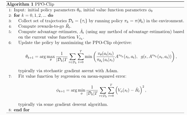
Proximal Policy Optimization (PPO) builds on policy gradient methods by improving stability and sample efficiency. It addresses large, destabilizing policy updates through mechanisms like clipped objectives or KL penalties. By combining gradient-based learning with divergence-based trust regions, PPO strikes a practical balance between exploration and stability, outperforming many earlier policy gradient algorithms.

• Pseudocode

• Example: Cartpole Balancing ( cartpole-dqn-ddpg-ppo)

Below is the walk through of some key implementation details of using PPO algorithms to sovle cartpole balancing task in Isaac Gym simulator.

• Policy Network and Value Network Definition

  class PPOPolicyNetwork(nn.Module):
      """
      Continuous action policy network.
      """
      def __init__(self, num_obs: int = 4, num_act: int = 1, hidden_size: int = 256):
          super(PPOPolicyNetwork, self).__init__()
  
          self.backbone = nn.Sequential(
              nn.Linear(num_obs, hidden_size),
              nn.LeakyReLU(),
              nn.Linear(hidden_size, hidden_size),
              nn.LeakyReLU(),
          )
          # Mean head
          self.mean_head = nn.Sequential(
              nn.Linear(hidden_size, num_act),
              nn.Tanh()             # action space is normalized to [-1,1]
          )
  
      def forward(self, x: torch.Tensor):
          """
          :param x:    Tensor of shape [batch_size, num_obs]
          :returns:    mean Tensor [batch_size, num_act],
                      std Tensor [num_act] (broadcastable over batch)
          """
          features = self.backbone(x)
          mean = self.mean_head(features)
          return mean
  
  class PPOValueNetwork(nn.Module):
      """
      State‐value function approximator.
      Outputs a single scalar V(x) per input state.
      """
      def __init__(self, num_obs: int = 4, hidden_size: int = 256):
          super(PPOValueNetwork, self).__init__()
          self.net = nn.Sequential(
              nn.Linear(num_obs, hidden_size),
              nn.LeakyReLU(),
              nn.Linear(hidden_size, hidden_size),
              nn.LeakyReLU(),
              nn.Linear(hidden_size, 1)
          )
  
      def forward(self, x: torch.Tensor):
          """
          :param x:  Tensor of shape [batch_size, num_obs]
          :returns:  V(x) Tensor of shape [batch_size, 1]
          """
          return self.net(x)    
  

  Note that policy network only outputs a mean \(\mu\), and here we build a Gaussian via a scheduled standard deviation \(\sigma\). Many continuous-control PPO implementations use fix or decay the log-std over training, rather than learning it. This reduces the number of trainable parameters and can make exploration more predictable, as long as make sure that early in training there is enough exploration (large \(\sigma\)), and later anneal toward more deterministic policies.

• get_action function

  As mentioned previously, the standard deviation of the action is scheduled in the main training scripts as follows:

  agent.action_var = torch.max(0.01 * torch.ones_like(agent.action_var), agent.action_var - 0.00002)
  

  Subsequently, the actions are sampled from the corresponding distribution (mean \(\mu\) predicted from policy network and standard deviation \(\sigma\) from schedule) by using the following function:

  def get_action(self, obs):
        with torch.no_grad():
            mu = self.policy_network(obs)
            cov_mat = torch.diag(self.action_var)
            dist = MultivariateNormal(mu, cov_mat)
            action = dist.sample()
            log_prob = dist.log_prob(action)
            action = action.clip(-1, 1)
        return action, log_prob
  

• make_data function

  This function gathers rollouts into minibatches and computes, for each time step, the TD-target, temporal-difference error (\(\delta\)), and generalized advantage estimate (GAE). It returns a list of tuples: (obs, action, old_log_prob, target, advantage) ready for PPO updates. The reversed loop implements backward-accumulation of GAE.

  def make_data(self):
    # organise data and make batch
    data = []
    for _ in range(self.chunk_size):
        obs_lst, a_lst, r_lst, next_obs_lst, log_prob_lst, done_lst = [], [], [], [], [], []
        for _ in range(self.mini_chunk_size):
            rollout = self.data.pop(0)
            obs, action, reward, next_obs, log_prob, done = rollout
  
            obs_lst.append(obs)
            a_lst.append(action)
            r_lst.append(reward.unsqueeze(-1))
            next_obs_lst.append(next_obs)
            log_prob_lst.append(log_prob)
            done_lst.append(done.unsqueeze(-1))
  
        obs, action, reward, next_obs, done = \
            torch.stack(obs_lst), torch.stack(a_lst), torch.stack(r_lst), torch.stack(next_obs_lst), torch.stack(done_lst)
  
        # compute reward-to-go (target)
        with torch.no_grad():
            target = reward + self.gamma * self.value_network(next_obs) * done
            delta = target - self.value_network(obs)
  
        # compute advantage
        advantage_lst = []
        advantage = 0.0
        for delta_t in reversed(delta):
            advantage = self.gamma * self.lmbda * advantage + delta_t
            advantage_lst.insert(0, advantage)
  
        advantage = torch.stack(advantage_lst)
        log_prob = torch.stack(log_prob_lst)
  
        mini_batch = (obs, action, log_prob, target, advantage)
        data.append(mini_batch)
    return data
  

  • target is defined as:

    \[T_t = r_t + \gamma V_\phi(s_{t+1})\]

    (masked by done so that terminal states don’t bootstrap).

  • delta is the one-step temporal difference:

    \[\delta_t = T_t - V_\phi(s_t)\]

  • This reversed loop implements:

    \[A_t = \sum_{l=0}^{T - t - 1} (\gamma \lambda)^l \delta_{t+l}\]

    accumulating from the end of the trajectory backward to reduce variance while retaining bias control — that’s GAE.

• update function (for both policy and value network)

  To update both policy and value neural networks, this function iterates over the collected mini-batches, recomputes action-log-probs under the current policy, forms the probability ratio, and builds two surrogate objectives: \(\text{surr1}\) and \(\text{surr2}\). The goal of updating policy network is to minimize the negative clipped surrogate for the policy and an MSE value loss, performing gradient ascent on the PPO objective.

• old_log_prob comes from data collected under \(\pi_{\theta_{\text{old}}}\)

• The ratio is:

  \[r_t(\theta) = \frac{\pi_\theta(a_t \mid s_t)}{\pi_{\theta_{\text{old}}}(a_t \mid s_t)}\]

  Equivalently, for each timestep \(t\):

  \[\text{surr1}_t = r_t(\theta) A_t,\] \[\text{surr2}_t = \text{clip}(r_t(\theta),\ 1 - \varepsilon,\ 1 + \varepsilon) A_t\]

• The inner min implements:

  \[L^{\text{clip}}(\theta) = \mathbb{E} \left[ \min(\text{surr1}_t,\ \text{surr2}_t) \right]\]
• The negative sign converts PPO’s maximization of \(L^{\text{clip}}\) into a minimization for standard optimizers.
• MSE loss is used for updating the value networks here, which aims to minimize the deviation from the value network prediction and calculated result from GAE.

    def update(self):
      # update actor and critic network
      data = self.make_data()

      for i in range(self.epoch):
          for mini_batch in data:
              obs, action, old_log_prob, target, advantage = mini_batch

              mu = self.policy_network(obs)
              cov_mat = torch.diag(self.action_var)
              dist = MultivariateNormal(mu, cov_mat)
              log_prob = dist.log_prob(action)

              ratio = torch.exp(log_prob - old_log_prob).unsqueeze(-1)

              surr1 = ratio * advantage
              surr2 = torch.clamp(ratio, 1 - self.clip, 1 + self.clip) * advantage

              loss_policy = -torch.min(surr1, surr2)
              loss_value = F.mse_loss(self.value_network(obs), target)

              self.policy_network.zero_grad(); self.value_network.zero_grad()
              loss_policy.mean().backward(); loss_value.mean().backward()
              nn.utils.clip_grad_norm_(self.policy_network.parameters(), 1.0)
              nn.utils.clip_grad_norm_(self.value_network.parameters(), 1.0)
              self.policy_optim.step(); self.value_optim.step()

              self.optim_step += 1

• old_log_prob comes from data collected under \(\pi_{\theta_{\text{old}}}\)

• The ratio is:

  \[r_t(\theta) = \frac{\pi_\theta(a_t \mid s_t)}{\pi_{\theta_{\text{old}}}(a_t \mid s_t)}\]

• Two surrogates:

  Equivalently, for each timestep \(t\):

  \[\text{surr1}_t = r_t(\theta) A_t,\] \[\text{surr2}_t = \text{clip}(r_t(\theta),\ 1 - \varepsilon,\ 1 + \varepsilon) A_t\]

• The inner min implements:

  \[L^{\text{clip}}(\theta) = \mathbb{E} \left[ \min(\text{surr1}_t,\ \text{surr2}_t) \right]\]
  • The negative sign converts PPO’s maximization of \(L^{\text{clip}}\) into a minimization for standard optimizers.

Summary

PPO enhances learning stability by clipping policy updates to prevent drastic jumps, effectively imposing a soft trust region without complex constraints. It also incorporates a generalized advantage estimator that smoothly blends short‐term and long‐term value estimates, reducing variance while maintaining low bias and greatly improving sample efficiency. PPO has been widely used in many domains:

• Legged Locomotion & Balancing
  PPO has become a de facto standard for training continuous-control policies on high-DoF robots, from simulating humanoid walking and running to stabilizing quadrupeds over uneven terrain.

• Imitation Learning & Sim-to-Real Transfer
  Many work combine the use of PPO with the learning of proprioceptive information and latent space representation such as this work for dexterous hand in-hand object orientation. There are also works on combining imitation learning with RL.

• Natural Language & RL from Human Feedback (RLHF)
  In large-language-model fine-tuning, PPO is used to optimize against learned reward models (e.g., human preference scorers), aligning model outputs with human values and stylistic constraints.

References

1. REINFORCE: Reinforcement Learning Most Fundamental Algorithm
2. Proximal Policy Optimization (OpenAI Spinning Up)
3. Overview of Deep Reinforcement Learning Methods
4. CS 182: Lecture 15: Part 1: Policy Gradients & Part 2 & Part 3 (Part of CS 182 from UC Berkeley)
5. The KL Divergence : Data Science Basics & Importance Sampling
6. minimal-isaac-gym, minimal-stable-PPO