
Interpreting LQR through Optimal Control and Reinforcement Learning
Published:
Linear Quadratic Regulator (LQR) is one the simplest yet most classical probelms in optimal control. While previous blog posts discussed the LQR optimal control law through Pontryagin’s Minimum Principle and Hamilton-Jacobi-Bellman Equation, This post approaches LQR from the perspective of Dynamic Programming and Reinforcement Learning (RL). In particular, it shows how LQR can be solved in a model-based setting using both policy iteration and value iteration, and how related ideas extend to model-free methods through temporal difference learning. Code accompanying the post is available in this repository.
This post is based primarily on the paper “Reinforcement Learning and Feedback Control” [1]. For a broader discussion and more technical detail, I recommend consulting the original paper.
1. Linear Quadratic Regulator
We begin with the discrete-time linear quadratic regulator (LQR), one of the canonical problems in optimal control. Its standard formulation is
\[\begin{aligned} \min_{\{u_k\}_{k=0}^{\infty}} \quad & J(x_0,\{u_k\}) = \frac{1}{2}\sum_{k=0}^{\infty}\left(x_k^\top Q x_k + u_k^\top R u_k\right) \\ \text{s.t.} \quad & x_{k+1} = A x_k + B u_k, \\ & x_0 \in \mathcal{X}. \end{aligned}\]Here, \(x_k \in \mathbb{R}^n\) is the state, \(u_k \in \mathbb{R}^m\) is the control input, \(Q \succeq 0 , R \succ 0\) are the matrices for state and control penalty respectively, and \(\mathcal{X}\) denotes the admissible set of initial states. The goal is to find a control sequence, or equivalently a feedback policy \(u_k = \pi(x_k)\), that stabilizes the system while minimizing the infinite-horizon quadratic cost.
In this post, let’s focus on a simple but representative example: a 2D double integrator. This system is especially useful because it is easy to interpret physically, yet rich enough to illustrate the main ideas behind optimal control.
1.1 Problem Formulation
The system considered here is a continuous-time double integrator with state \(x = [p, v]^\top\), where \(p\) denotes position and \(v\) denotes velocity, and control input \(u \in \mathbb{R}\). Its continuous-time dynamics are
\[\dot{x} = A_c x + B_c u,\]with
\[A_c = \begin{bmatrix} 0 & 1 \\ 0 & 0 \end{bmatrix}, \qquad B_c = \begin{bmatrix} 0 \\ 1 \end{bmatrix}.\]This is the standard point-mass model in which the control acts as acceleration: position integrates velocity, and velocity integrates the input.
The simulation is carried out in discrete time, and the sampling time is chosen to be \(\Delta t = 0.02 \text{ s}.\) Under zero-order hold, the input is assumed constant over each sampling interval. Implementation detail can be found here in the code.
The finite simulation horizon is chosen as
\[T_{\text{final}} = 5.0 \text{ s},\]and the initial condition is
\[x_0 = \begin{bmatrix} 1.0 \\ 0.0 \end{bmatrix},\]meaning that the system starts one unit away from the origin with zero initial velocity.
Following the control objective defined previously in the canonical LQR, the weighting matrices are
\[Q = \begin{bmatrix} 10.0 & 0 \\ 0 & 1.0 \end{bmatrix}, \qquad R = \begin{bmatrix} 0.1 \end{bmatrix}.\]These choices penalize position error more heavily than velocity error, while assigning a moderate penalty to control effort. As a result, the controller is encouraged to regulate the position quickly without using unnecessarily aggressive inputs.
The goal is to compute a feedback policy of the form
\[u_k = \pi(x_k),\]and, for the LQR case, this policy takes the familiar linear form
\[u_k = -Kx_k.\]This concrete setup will be used throughout the rest of the post when discussing the solution method, numerical implementation, and the connection between the theory and the code.
1.2 A Bridge to Dynamic Programming
LQR is usually introduced through a state-space model,
\[x_{k+1} = A x_k + B u_k,\]which is the standard language of control theory. This viewpoint emphasizes system dynamics, feedback, and controller design for a known plant.
Dynamic programming and reinforcement learning often use a different modeling language, namely the Markov decision process (MDP). An MDP is specified by states, actions, transition laws, and one-step costs or rewards. From this perspective, a control problem is viewed as a sequential decision problem in which each action affects both the immediate cost and the distribution of future states.
These two viewpoints describe the same underlying problem at different levels. The state-space model is the natural starting point in control, while the MDP formulation is convenient for expressing value functions and Bellman equations. In deterministic systems such as discrete-time LQR, the state equation induces a degenerate transition law: once \(x_k\) and \(u_k\) are fixed, the next state is uniquely determined. This makes LQR a natural bridge between optimal control and reinforcement learning.
With this connection in place, we now turn to dynamic programming, which provides the recursive framework underlying both optimal control and reinforcement learning.
2. Dynamic Programming
2.1 Problem Formulation
Dynamic programming studies optimal sequential decision making over time. In the setting used in the paper, the problem is formulated as a Markov decision process (MDP), where at each stage \(k\), the system is in state \(x_k\), an action \(u_k\) is selected, and the system transitions to the next state \(x_{k+1}\). The transition law is described by the conditional probability
\[P^u_{x,x'} = \Pr(x_{k+1}=x' \mid x_k=x,\; u_k=u),\]and the one-step cost is written as \(r_k = r(x_k,u_k,x_{k+1})\), or equivalently through its conditional expectation \(R^u_{x,x'}\).
A standard infinite-horizon dynamic-programming objective is to minimize the discounted cumulative cost
\[J_k = \sum_{i=0}^{\infty} \gamma^i r_{k+i},\]where \(0 \le \gamma < 1\) is the discount factor. The role of \(\gamma\) is to reduce the weight of costs incurred further in the future and to ensure that the infinite sum is well behaved.
This is the standard formulation in dynamic programming and reinforcement learning, but it is not exactly the same as the usual infinite-horizon LQR problem. In standard LQR, one typically starts from a deterministic state-space model and an undiscounted quadratic cost. If one introduces a discount factor \(\gamma < 1\) into LQR, then one is solving a discounted optimal control problem, rather than the standard LQR formulation that leads to the algebraic Riccati equation. Since our goal later is to study policy iteration, value iteration, and the ARE in the LQR setting, the relevant dynamic-programming viewpoint for LQR is the undiscounted one, even though the discounted formulation is the more common generic template in MDPs.
2.2 The Value Function
The central object in dynamic programming is the value function. For a fixed policy \(\pi\), the value function \(V^\pi(x)\) is the expected cumulative future cost when the system starts at state \(x\) and follows \(\pi\) thereafter. In the notation used in the paper, this is written as
\[V^\pi(x) = \sum_u \pi(x,u)\sum_{x'} P^u_{x,x'} \left[ R^u_{x,x'}+\gamma V^\pi(x') \right].\]This expression is worth unpacking carefully. The outer summation,
\[\sum_u \pi(x,u)(\cdot),\]averages over all actions that may be taken at state \(x\). Here, \(\pi(x,u)\) is the probability of choosing action \(u\) when the current state is \(x\) . If the policy is stochastic, several actions may have nonzero probability; if the policy is deterministic, all probability mass is concentrated on a single action.
For each chosen action \(u\), the inner summation,
\[\sum_{x'} P^u_{x,x'}(\cdot),\]averages over all possible next states \(x'\). The quantity \(P^u_{x,x'}\) is the probability that the next state becomes \(x'\) given that the current state is \(x\) and action \(u\) is applied . This term encodes the system dynamics in probabilistic form.
Inside the brackets,
\[R^u_{x,x'}+\gamma V^\pi(x'),\]the term \(R^u_{x,x'}\) is the immediate one-step cost associated with the transition from \(x\) to \(x'\) under action \(u\), while \(\gamma V^\pi(x')\) is the discounted future cost-to-go after the system arrives at state \(x'\). Thus, the bracketed term represents the total contribution of one transition: immediate cost plus future cost.
Putting these pieces together, the value function is computed by a two-level averaging process. First, for a fixed action, one averages over all possible next states using the transition probabilities. Then one averages over all possible actions using the policy probabilities. In this sense, the value function is a conditional expectation of immediate cost plus discounted future cost.
The value function is policy-dependent, while the optimal value function is policy-independent. This distinction is important:
\(V^\pi(x)\) evaluates the long-term performance of a particular policy \(\pi\), whereas \(V^*(x)\) describes the best achievable cost-to-go regardless of which policy attains it.
For deterministic dynamics,
\[x_{k+1}=f(x_k,u_k),\]the transition law simplifies to
\[P^u_{x,x'}= \begin{cases} 1, & x'=f(x,u),\\ 0, & \text{otherwise}. \end{cases}\]In that case, the sum over next states collapses because there is only one possible successor state. If the policy is also deterministic, then the sum over actions collapses as well, and the value function reduces to
\[\begin{array}{|c|} \hline V^\pi(x)=r(x,\pi(x))+\gamma V^\pi(f(x,\pi(x))). \\ \hline \end{array}\]Thus, the probabilistic MDP notation reduces to the familiar deterministic recursion from control.
2.3 Bellman Equation and Optimality
The Bellman equation is the basic recursive relation of dynamic programming. For a fixed policy \(\pi\), it states that the value at the current state equals the expected one-step cost plus the value of the next state:
\[V^\pi(x) = \sum_u \pi(x,u)\sum_{x'} P^u_{x,x'} \left[ R^u_{x,x'}+\gamma V^\pi(x') \right].\]This is a consistency relation: the cost-to-go from the current state must agree with the immediate cost incurred now plus the future cost-to-go from the next state.
The optimal value function \(V^*(x)\) is defined as the minimum achievable cost-to-go over all admissible policies. It satisfies the Bellman optimality equation
\[V^*(x) = \min_u \sum_{x'} P^u_{x,x'} \left[ R^u_{x,x'}+\gamma V^*(x') \right].\]Compared with the Bellman equation for a fixed policy, the policy probabilities \(\pi(x,u)\) are replaced by a minimization over actions. The meaning is straightforward: at each state, the optimal action is the one that minimizes the sum of immediate cost and future optimal cost.
This minimization is the mathematical expression of Bellman’s principle of optimality. Once the current decision is made optimally, the remaining decisions must also form an optimal strategy for the state reached next. In this way, a global sequential optimization problem is converted into a recursive local one.
In deterministic systems, the Bellman optimality equation simplifies to
\[\begin{array}{|c|} \hline \displaystyle V^*(x)=\min_u \left[r(x,u)+\gamma V^*(f(x,u))\right]. \\ \hline \end{array}\]The corresponding optimal action is obtained by taking the action that attains this minimum:
\[\begin{array}{|c|} \hline \displaystyle u^*(x)=\arg\min_u \left[r(x,u)+\gamma V^*(f(x,u))\right]. \\ \hline \end{array}\]Here there is no need to average over next states, since the next state is uniquely determined by the current state and action. The only remaining operation is the minimization over admissible actions.
2.4 Bellman Equation for Discrete-time LQR and the Lyapunov equation
A particularly important specialization of the Bellman equation arises in discrete-time LQR. In this setting, the dynamics are deterministic,
\[x_{k+1} = A x_k + B u_k,\]and the infinite-horizon performance index is written as
\[J_k = \frac{1}{2}\sum_{i=k}^{\infty} r_i = \frac{1}{2}\sum_{i=k}^{\infty}\left(x_i^\top Q x_i + u_i^\top R u_i\right).\]Accordingly, for a stationary policy \(u_k=\mu(x_k)\), the associated value function is
\[V(x_k)=\frac{1}{2}\sum_{i=k}^{\infty}\left(x_i^\top Q x_i + u_i^\top R u_i\right).\]Under this formulation, the Bellman equation for a fixed policy takes the form
\[V(x_k)=\frac{1}{2}\left(x_k^\top Q x_k + u_k^\top R u_k\right)+V(x_{k+1}).\]To specialize further to LQR, consider a stationary linear state-feedback controller
\[u_k=-Kx_k.\]The closed-loop dynamics are then
\[x_{k+1}=(A-BK)x_k.\]Now assume that the value function is quadratic,
\[\begin{array}{|c|} \hline \displaystyle V(x_k)=\frac{1}{2}x_k^\top P x_k, \\ \hline \end{array}\]for some symmetric matrix \(P\). Substituting this ansatz into the Bellman equation yields
\[x_k^\top P x_k = x_k^\top Q x_k + u_k^\top R u_k + x_{k+1}^\top P x_{k+1}.\]Using \(u_k=-Kx_k\) and \(x_{k+1}=(A-BK)x_k\) gives
\[x_k^\top P x_k = x_k^\top Q x_k + x_k^\top K^\top R K x_k + x_k^\top (A-BK)^\top P (A-BK)x_k.\]Since this identity holds for all \(x_k\), the corresponding quadratic forms must coincide, and therefore
\[P = Q + K^\top R K + (A-BK)^\top P (A-BK).\]Equivalently,
\[\begin{array}{|c|} \hline (A-BK)^\top P (A-BK) - P + Q + K^\top R K = 0. \\ \hline \end{array}\]This is a discrete-time Lyapunov equation with closed-loop matrix \(A_{\mathrm{cl}} = A-BK\) and stage-cost matrix \(Q_{\mathrm{cl}} = Q + K^\top R K\). Thus, policy evaluation for a given stabilizing linear controller reduces to solving a Lyapunov equation for the matrix \(P\) .
This equivalence is important for several reasons:
- it shows that, under a fixed stabilizing controller, the value function is exactly a quadratic function determined by a matrix equation;
- it makes the role of stability explicit, since a well-behaved solution \(P\) is tied to the stability of the closed-loop matrix \(A-BK\);
- it shows that the value function also serves as a Lyapunov-function candidate for the closed-loop system.
Indeed, along closed-loop trajectories,
\[V(x_k)-V(x_{k+1}) = \frac{1}{2}\left(x_k^\top Q x_k + u_k^\top R u_k\right)\ge 0,\]so the value decreases by exactly the stage cost at each step. This is precisely the monotonic decay property studied in Lyapunov theory.
It is also useful to distinguish this equation from the algebraic Riccati equation, which arises in the optimal-control setting discussed next. When the feedback gain \(K\) is fixed, the Bellman equation is linear in the unknown matrix \(P\), and the result is a Lyapunov equation. By contrast, when one starts from the Bellman optimality equation and minimizes over the control input, the minimization introduces a nonlinear dependence on \(P\), leading to the algebraic Riccati equation. In this sense,
policy evaluation for a fixed controller corresponds to a Lyapunov equation;
optimal control synthesis corresponds to a Riccati equation.
2.5 Algebraic Riccati Equation (ARE)
The Lyapunov equation in the previous subsection arises when the feedback policy is fixed. To derive the algebraic Riccati equation (ARE), one instead begins from the Bellman optimality equation, in which the control input is chosen to minimize the infinite-horizon cost. Recall the corresponding Bellman optimality equation for discrete time LQR can be written as
\[\begin{array}{|c|} \hline \displaystyle V^*(x)=\min_u \left[\frac{1}{2}\left(x^\top Q x + u^\top R u\right)+V^*(Ax+Bu)\right]. \\ \hline \end{array}\]As in the fixed-policy case, assume the optimal value function is quadratic:
\[V^*(x)=\frac{1}{2}x^\top P x,\]for some symmetric matrix \(P\). Substituting this ansatz into the Bellman optimality equation gives
\[\frac{1}{2}x^\top P x = \min_u \left[ \frac{1}{2}\left(x^\top Q x + u^\top R u\right) + \frac{1}{2}(Ax+Bu)^\top P (Ax+Bu) \right].\]Multiplying both sides by \(2\) yields
\[x^\top P x = \min_u \left[ x^\top Q x + u^\top R u + (Ax+Bu)^\top P (Ax+Bu) \right].\]The next step is to expand the quadratic term:
\[(Ax+Bu)^\top P (Ax+Bu) = x^\top A^\top P A x + 2x^\top A^\top P B u + u^\top B^\top P B u.\]Substituting this back into the Bellman equation gives
\[x^\top P x = \min_u \left[ x^\top (Q+A^\top P A)x + 2x^\top A^\top P B u + u^\top (R+B^\top P B)u \right].\]Now the right-hand side is a quadratic function of \(u\). The optimal control is obtained by minimizing this expression with respect to \(u\). Taking the derivative with respect to \(u\) and setting it equal to zero gives the first-order optimality condition
\[2(R+B^\top P B)u + 2B^\top P A x = 0,\]or equivalently,
\[(R+B^\top P B)u = -B^\top P A x.\]Assuming \(R+B^\top P B\) is invertible, the minimizing control is
\[u^* = -(R+B^\top P B)^{-1}B^\top P A x.\]Thus, the optimal controller has the linear state-feedback form
\[u^* = -Kx,\]with gain
\[\begin{array}{|c|} \hline \displaystyle K = (R+B^\top P B)^{-1}B^\top P A. \\ \hline \end{array}\]Let \(G = (R+B^\top P B)^{-1}\), and since \(R\) and \(P\) are symmetric, \(G\) is also symmetric. Thus, \((G ^{-1})^\top = (G^\top)^{-1} = G^{-1}\). Substituting this minimizing control back into the Bellman optimality equation yields the matrix equation satisfied by \(P\):
\[\begin{array}{|c|} \hline \textbf{Discrete-time ARE} \\ P = Q + A^\top P A - A^\top P B (R+B^\top P B)^{-1} B^\top P A. \\ \hline \end{array}\]It is useful to compare this with the Lyapunov equation from the previous subsection. For a fixed controller \(K\), one obtained
\[P = Q + K^\top R K + (A-BK)^\top P (A-BK),\]which is linear in \(P\) once \(K\) is fixed. In contrast, the Riccati equation contains the term
\[A^\top P B (R+B^\top P B)^{-1} B^\top P A,\]which depends nonlinearly on \(P\). This nonlinearity comes directly from eliminating the minimizing control \(u\). That is why the Bellman equation for a fixed policy becomes a Lyapunov equation, while the Bellman optimality equation becomes a Riccati equation .
This derivation also clarifies the relationship between policy evaluation and optimal synthesis. In policy evaluation, the control law is already known, and one solves for the value function under that policy.
In optimal synthesis, the control law is not known in advance; it must be found simultaneously with the value function by minimizing the Bellman equation. The Riccati equation is precisely the condition that makes this joint optimization possible in the linear-quadratic setting. In this way, the ARE plays the central role in infinite-horizon discrete-time LQR: it characterizes both the optimal value function and the optimal state-feedback controller.
3. Policy Iteration for Discrete-time LQR
Policy iteration solves the discrete-time LQR problem by alternating between policy evaluation and policy improvement. Rather than solving the algebraic Riccati equation directly, it starts from an initial stabilizing feedback gain \(K^0\), evaluates the cost of the current controller, and then updates the controller using the resulting value function.
Consider the discrete-time LQR system
\[x_{k+1}=Ax_k+Bu_k.\]At policy-iteration step \(j\), the controller is taken to be a linear feedback law
\[u_k^j=-K^j x_k,\]where \(j\) is the policy-iteration index, not the time index. The goal is to generate a sequence of gains \(K^0,K^1,K^2,\ldots\) that converges to the optimal LQR gain.
3.1 Policy Evaluation
The policy-evaluation step computes the value function associated with the current feedback gain \(K^j\). Since the policy is fixed, the Bellman equation reduces to a discrete-time Lyapunov equation:
\[P^j = Q + (K^j)^\top R K^j + (A-BK^j)^\top P^j (A-BK^j).\]Equivalently,
\[(A-BK^j)^\top P^j (A-BK^j) - P^j + Q + (K^j)^\top R K^j = 0.\]Solving this equation gives the quadratic value function for the current policy:
\[V^j(x)=\frac{1}{2}x^\top P^j x.\]This step only evaluates the current controller; it does not yet modify the policy. It answers the question: given \(K^j\), what is the infinite-horizon cost-to-go from each state?
For the evaluation to be well defined, the closed-loop matrix
\[A-BK^j\]must be stable, meaning that all its eigenvalues lie inside the unit circle. This is why policy iteration for LQR is typically initialized with a stabilizing gain \(K^0\). Under this condition, the Lyapunov equation has a finite solution \(P^j\), and the corresponding infinite-horizon cost is finite. In the corresponding repository, the code follwing is used for policy evaluation:
  import numpy as np
  from scipy.linalg import solve_discrete_are, solve_discrete_lyapunov
  def policy_evaluation(A: np.ndarray, B: np.ndarray, Q: np.ndarray, R: np.ndarray, K: np.ndarray):
       """
       Exact policy evaluation for a fixed linear policy u = -Kx.

       Solves:
            P = (A - BK)^T P (A - BK) + (Q + K^T R K)
       """
       A_cl = A - B @ K
       Q_cl = Q + K.T @ R @ K
       P = solve_discrete_lyapunov(A_cl.T, Q_cl)
       return symmetrize(P)
3.2 Policy Improvement
After computing \(P^j\), the policy-improvement step updates the controller by choosing the action that minimizes the one-step lookahead cost. Using the current value function \(V^j(x)=\frac{1}{2}x^\top P^j x\), the improved policy is defined by
\[\mu^{j+1}(x) = \arg\min_u \left[ x^\top Qx + u^\top Ru + (Ax+Bu)^\top P^j(Ax+Bu) \right].\]This expression is the LQR version of the greedy improvement step: it chooses the control \(u\) that minimizes the current stage cost plus the estimated future cost under the value matrix \(P^j\). In this sense, the term
\[x^\top Qx + u^\top Ru + (Ax+Bu)^\top P^j(Ax+Bu)\]is the one-step lookahead cost .
Solving the minimization gives a linear feedback policy
\[\mu^{j+1}(x)=-K^{j+1}x,\]where
\[\begin{array}{|c|} \hline \displaystyle K^{\color{red}{j+1}} = \left(B^\top P^j B + R\right)^{-1}B^\top P^j A. \\ \hline \end{array}\]Thus, policy improvement uses the value matrix from the current policy to construct a new greedy controller . Under the standard assumptions and with a stabilizing initialization, this new policy is no worse than the previous one. In terms of value functions,
\[V^{j+1}(x)\le V^j(x),\]or equivalently, in terms of value matrices,
\[P^{j+1}\preceq P^j.\]The algorithm repeats policy evaluation and policy improvement until the gain or value matrix changes only slightly, for example when
\[\|P^{j+1}-P^j\|<\varepsilon\]or
\[\|K^{j+1}-K^j\|<\varepsilon\]for some tolerance \(\varepsilon>0\). At convergence, \(K^{j+1}\approx K^j\), and the limiting value matrix satisfies the algebraic Riccati equation.
In short, policy iteration alternates between solving a Lyapunov equation for the current gain and applying a greedy one-step improvement. With a stabilizing initialization, this process converges to the optimal LQR value matrix \(P^*\) and feedback gain \(K^*\). The following code is used for policy improvement:
  def policy_improvement(A: np.ndarray, B: np.ndarray, R: np.ndarray, P: np.ndarray) -> np.ndarray:
       """
       Greedy / policy-improvement step for discrete-time LQR.

       For a quadratic value matrix P, return the improved linear feedback gain K
       for u_k = -K x_k.
       """
       G = R + B.T @ P @ B
       F = B.T @ P @ A
       K = np.linalg.solve(G, F)
       return K
3.3 Results
The following implementation is used for conducting policy iteration to solve LQR problem:
   def policy_iteration(A: np.ndarray, B: np.ndarray, Q: np.ndarray, R: np.ndarray,
             K0: np.ndarray, max_iters: int = 200, tol: float = 1e-10):
        K = K0.copy()
        last_delta_P = np.inf
        last_delta_K = np.inf
        converged = False

        for it in range(1, max_iters + 1):
             P = policy_evaluation(A, B, Q, R, K)
             K_new = policy_improvement(A, B, R, P)

             P_new = policy_evaluation(A, B, Q, R, K_new)

             last_delta_P = np.linalg.norm(P_new - P, ord="fro")
             last_delta_K = np.linalg.norm(K_new - K, ord="fro")

             K = K_new
             P = P_new

             if max(last_delta_P, last_delta_K) < tol:
                  converged = True
                  break

        eig_closed_loop = np.linalg.eigvals(A - B @ K)
        return {
             "P": P,
             "K": K,
             "iterations": it,
             "converged": converged,
             "last_delta_P": last_delta_P,
             "last_delta_K": last_delta_K,
             "eig_closed_loop": eig_closed_loop,
        }
and the result are as follows:
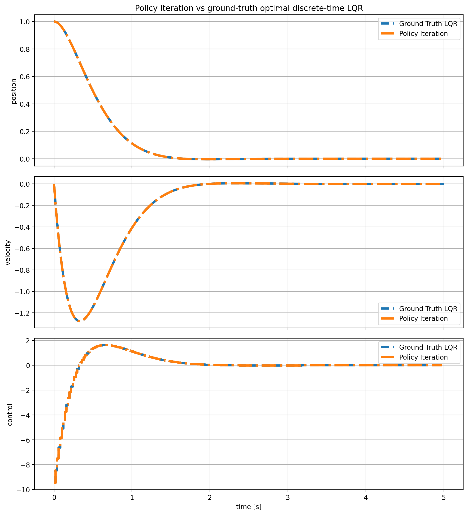
Policy Iteration Result.
4. Value Iteration for Discrete-time LQR
Value iteration provides a second dynamic-programming route to the discrete-time LQR problem. Like policy iteration, it is based on Bellman’s recursion, but the update mechanism is different. Policy iteration evaluates the current policy exactly before improving it, whereas value iteration performs only a single Bellman-style update of the value function at each step and then updates the policy accordingly. In this sense, value iteration may be viewed as a more direct fixed-point iteration on the Bellman optimality equation.
In the LQR setting, it is natural to represent the value function at iteration \(j\) in quadratic form,
\[V^j(x)=\frac{1}{2}x^\top P^j x,\]where \(P^j\) is the value matrix at iteration \(j\). The value-iteration algorithm then produces a sequence of matrices \(P^0,P^1,P^2,\dots\) together with a sequence of feedback gains \(K^0,K^1,K^2,\dots\).
A useful way to understand the difference from policy iteration is the following. In policy iteration, the policy-evaluation step solves a Lyapunov equation exactly for the current controller \(K^j\), and only then updates the policy. In value iteration, one does not solve the full policy-evaluation equation at each step. Instead, one performs a single recursion step toward the value of the current policy, and then immediately updates the control law. As a result, value iteration is often simpler per iteration, though it usually requires more iterations overall.
4.1 Value Update
The value-update step applies one Bellman recursion to the current value estimate. In a general dynamic-programming setting, value iteration replaces exact policy evaluation by a one-step update of the value function. In the discrete-time LQR setting, this takes a particularly simple quadratic form.
Suppose the current controller is
\[u_k^j=-K^j x_k,\]and the current value estimate is represented by
\[V^j(x)=\frac{1}{2}x^\top P^j x.\]Then the next value iterate is obtained from the Bellman recursion
\[\begin{array}{|c|} \hline \displaystyle V^{\color{red}{j+1}}(x_k) = \frac{1}{2}\left(x_k^\top Qx_k + (u_k^j)^\top R u_k^j\right) + V^j(x_{k+1}), \\ \hline \end{array}\]where
\[x_{k+1}=Ax_k+Bu_k^j.\]Substituting the linear feedback law \(u_k^j=-K^j x_k\) and the quadratic value approximation gives the matrix recursion
\[\begin{array}{|c|} \hline \displaystyle P^{\color{red}{j+1}} = (A-BK^j)^\top P^j (A-BK^j) + Q + (K^j)^\top R K^j. \\ \hline \end{array}\]This recursion is closely related to the Lyapunov equation from policy evaluation, but it is not the same. In policy iteration, one solves
\[P^j = (A-BK^j)^\top P^j (A-BK^j) + Q + (K^j)^\top R K^j\]exactly for \(P^j\). In value iteration, by contrast, one updates \(P^{j+1}\) from the previous matrix \(P^j\) using a single recursion step . Thus, value iteration replaces exact policy evaluation by an iterative value update.
This viewpoint is important conceptually. The matrix \(P^{j+1}\) should be interpreted as a refined estimate of the cost-to-go, obtained by taking the current stage cost and adding the previous estimate of the future cost. It is therefore an approximation step toward the fixed point that satisfies the Bellman equation.
In the LQR setting, the value-update step can also be understood as a Lyapunov recursion. For a fixed gain \(K^j\), the map
\[P^j \mapsto P^{j+1} = (A-BK^j)^\top P^j (A-BK^j) + Q + (K^j)^\top R K^j\]is precisely the one-step Lyapunov update associated with the closed-loop system. This is one reason value iteration fits naturally into the control interpretation of Bellman’s equation.
4.2 Policy Improvement
Once the updated value matrix \(P^{j+1}\) has been computed, the controller is improved by minimizing the one-step lookahead cost with respect to the control input. As in policy iteration, this is a greedy Bellman improvement step, but now it uses the newly updated value matrix \(P^{j+1}\) rather than the exact value of the current policy.
The policy-improvement step is therefore
\[\mu^{j+1}(x) = \arg\min_u \left[ x^\top Qx + u^\top Ru + (Ax+Bu)^\top P^{j+1}(Ax+Bu) \right].\]Solving this minimization yields the updated linear feedback law
\[\mu^{j+1}(x)=-K^{j+1}x,\]with gain
\[\begin{array}{|c|} \hline \displaystyle K^{j+1} = \left(B^\top P^{j+1}B+R\right)^{-1}B^\top P^{j+1}A. \\ \hline \end{array}\]Thus, the value-iteration loop alternates between two operations:
- update the value matrix using one Bellman/Lyapunov recursion step;
- update the feedback gain by minimizing the resulting one-step lookahead cost.
Compared with policy iteration, the key distinction is that the value matrix used in the improvement step is not obtained by exact policy evaluation. It is only the next value iterate. For this reason, value iteration is often interpreted as an approximate form of policy iteration in which the policy-evaluation phase has been truncated to a single step. Unlike policy iteration, value iteration does not require that initial gain be stabilizing and can be initialized with any feedback gain.
4.3 Results
The following implementation is used for conducting value iteration to solve LQR problem:
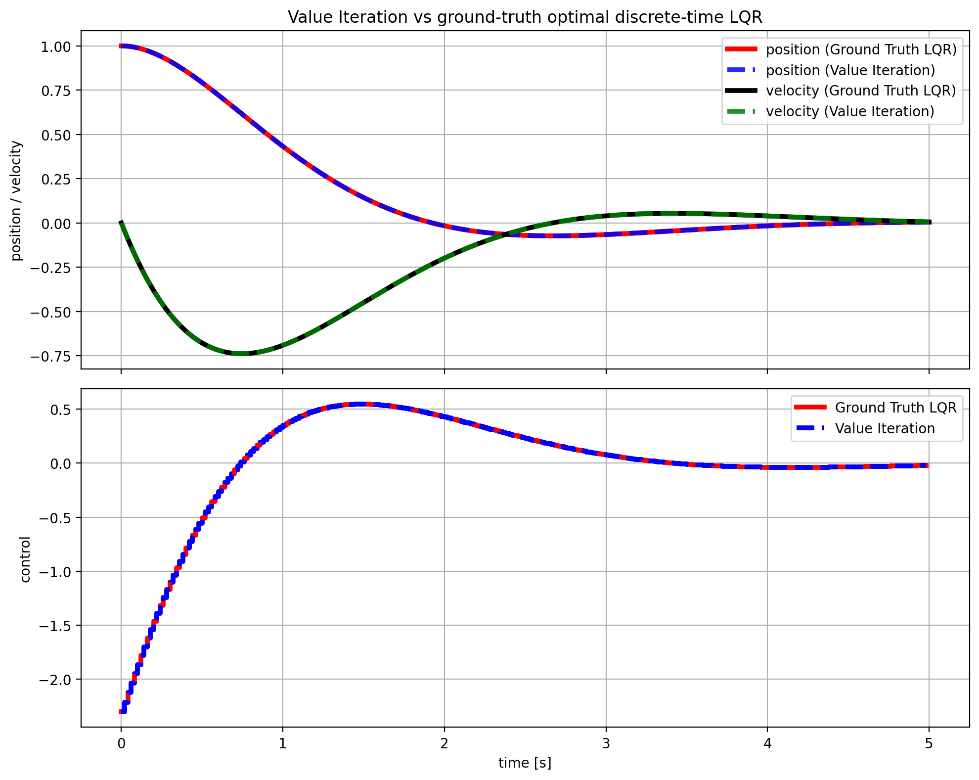
   def value_iteration(A: np.ndarray, B: np.ndarray, Q: np.ndarray, R: np.ndarray,
             P0: np.ndarray, max_iters: int = 200, tol: float = 1e-10):
        P = symmetrize(P0.copy())
        last_delta_P = np.inf
        last_delta_K = np.inf
        converged = False
        K_prev = np.zeros((B.shape[1], A.shape[0]))

        for it in range(1, max_iters + 1):
             G = R + B.T @ P @ B
             H = B.T @ P @ A

             P_new = Q + A.T @ P @ A - A.T @ P @ B @ np.linalg.solve(G, H)
             P_new = symmetrize(P_new)

             K_new = policy_improvement(A, B, R, P_new)

             last_delta_P = np.linalg.norm(P_new - P, ord="fro")
             last_delta_K = np.linalg.norm(K_new - K_prev, ord="fro")

             P = P_new
             K_prev = K_new

             if max(last_delta_P, last_delta_K) < tol:
                  converged = True
                  break

        eig_closed_loop = np.linalg.eigvals(A - B @ K_prev)
        return {
             "P": P,
             "K": K_prev,
             "iterations": it,
             "converged": converged,
             "last_delta_P": last_delta_P,
             "last_delta_K": last_delta_K,
             "eig_closed_loop": eig_closed_loop,
        }
and the result are as follows:

Value Iteration Result.
5. Model-free Q learning for Solving LQR
So far, the discussion has focused on dynamic-programming methods that assume the system model is known. In discrete-time LQR, this means knowing the matrices \(A\) and \(B\), so that Bellman updates, policy iteration, and value iteration can be written explicitly in terms of the state transition
\[x_{k+1}=Ax_k+Bu_k.\]From that viewpoint, the optimal controller is obtained through matrix equations such as the Lyapunov equation or the algebraic Riccati equation.
A natural next question is whether one can recover the same optimal controller without knowing the system matrices in advance. This is precisely the model-free viewpoint. Rather than starting from an explicit state-space model, model-free methods seek to learn the quantities needed for control directly from data collected along system trajectories. In the reinforcement-learning language, the key object for doing this is not only the value function, but also the Q function, or action-value function.
The reason the Q function is useful is that it evaluates a state-action pair directly. The value function \(V(x)\) tells us the long-term cost starting from state \(x\) once a policy has already selected an action. By contrast, the Q function \(Q(x,u)\) tells us the long-term cost of taking a specific action \(u\) at state \(x\), and then following a policy afterward . This extra dependence on the action is important in model-free settings, because it allows policy improvement to be expressed directly as a minimization of the Q function, without first needing explicit knowledge of the system dynamics.
5.1 Q Function
To move toward model-free methods, it is useful to introduce the Q function, also called the action-value function. In the dynamic-programming formulation, the value function \(V^\pi(x_k)\) measures the expected future cost when the system starts at state \(x_k\) and follows the policy \(\pi\) thereafter. The Q function refines this idea by also keeping track of the control action taken at the current step. It measures the cost of applying a specific control \(u_k\) at the current state \(x_k\), and then following the policy \(\pi\) from time \(k+1\) onward.
In the notation of the paper, the infinite-horizon Q function for a fixed policy \(\pi\) is written as
\[Q^\pi(x_k,u_k)=\sum_{x_{k+1}} P^{u_k}_{x_k,x_{k+1}} \left[ R^{u_k}_{x_k,x_{k+1}}+\gamma V^\pi(x_{k+1}) \right].\]This is the quantity that appears in equation (37). Its meaning is straightforward: starting from the pair \((x_k,u_k)\), one first incurs the immediate one-step cost, then moves to the next state \(x_{k+1}\), and then accumulates the remaining cost according to the value function of the policy \(\pi\). Thus, \(Q^\pi(x_k,u_k)\) is the cost of taking a prescribed action now and following the fixed policy afterward.
For discrete-time LQR, the dynamics are deterministic, so there is no need to average over multiple next states. In that case, equation (37) simplifies to
\[Q^\pi(x_k,u_k) = \frac{1}{2}\left(x_k^\top Qx_k+u_k^\top Ru_k\right) + V^\pi(x_{k+1}), \qquad x_{k+1}=Ax_k+Bu_k.\]This form is especially intuitive in the LQR setting: the Q function is simply the current quadratic stage cost plus the value of the next state, where the next state is generated by the current control input.
The phrase fixed policy means that the policy \(\pi\) is held fixed during evaluation. One is not yet optimizing over all future decisions. Instead, one asks the following question: if the current state is \(x_k\), and an arbitrary action \(u_k\) is applied now, but from the next time onward the controller reverts to the policy \(\pi\), what total cost will be incurred? That is exactly what \(Q^\pi(x_k,u_k)\) measures. So the current action \(u_k\) is free, but all subsequent actions are determined by the fixed policy \(\pi\).
Once the Q function is defined, the value function is recovered by evaluating the Q function at the action chosen by the policy . This is the meaning of equation (38):
\[V^\pi(x_k)=Q^\pi(x_k,\pi(x_k)).\]In words, the value at state \(x_k\) is the Q value of the state-action pair obtained when the policy selects the control \(u_k=\pi(x_k)\). Equation (37) therefore tells us how to evaluate an arbitrary current action followed by \(\pi\), while equation (38) says that the value function is the special case in which the current action is exactly the one prescribed by the policy. Subsequently, the Q function Bellman equation in the deterministic setting can be written as:
\[\begin{array}{|c|} \hline \displaystyle Q^\pi(x_k, u_k)= r(x_k, u_k) + \gamma Q^\pi(x_{k+1},\pi(x_{k+1})). \\ \hline \end{array}\]The paper also defines the optimal Q function, denoted by \(Q_k^*(x_k,u_k)\). It is the conditional expected cost obtained by taking action \(u_k\) at state \(x_k\) and then following an optimal policy thereafter:
\[Q_k^*(x_k,u_k) = \mathbb{E}_\pi \left\{ r_k+\gamma V_{k+1}^*(x_{k+1}) \mid x_k=x,\;u_k=u \right\}.\]In the stochastic setting, this can also be written as
\[Q_k^*(x_k,u_k) = \sum_{x_{k+1}} P^{u_k}_{x_k,x_{k+1}} \left[ R^{u_k}_{x_k,x_{k+1}}+\gamma V_{k+1}^*(x_{k+1}) \right].\]This is the content of equation (32) in the paper. The key point is that \(Q_k^*\) is no longer tied to a prescribed policy \(\pi\). Instead, it measures the cost of taking a current action and then behaving optimally from the next step onward.
In terms of the optimal Q function, the Bellman optimality equation takes the particularly simple form
\[\begin{array}{|c|} \hline \displaystyle V_k^*(x_k)=\min_{u_k} Q_k^*(x_k,u_k),\\ \hline \end{array}\]which is equation (33) in the paper. This equation says that the optimal value at a state is obtained by choosing the action that minimizes the optimal Q function. This is one of the main reasons the Q function is so useful: policy improvement can be carried out directly by minimizing over the action variable.
In the LQR setting, the policy is linear, and the value function is quadratic,
\[\pi(x_k)=-Kx_k,\] \[V^\pi(x_k)=\frac{1}{2}x_k^\top P x_k,\]then the Q function is also quadratic. Substituting \(x_{k+1}=Ax_k+Bu_k\) into the deterministic form of equation (37) gives
\[Q^\pi(x_k,u_k) = \frac{1}{2}\left(x_k^\top Qx_k+u_k^\top Ru_k\right) + \frac{1}{2}(Ax_k+Bu_k)^\top P (Ax_k+Bu_k).\]With \(P\) being the Riccati solution, the Q function for the discrete-time LQR can be written as
\[\begin{array}{|c|} \hline \displaystyle Q(x_k,u_k) = \frac{1}{2} \begin{bmatrix} x_k\\ u_k \end{bmatrix}^{\!\top} \begin{bmatrix} A^\top P A + Q & B^\top P A\\ A^\top P B & B^\top P B + R \end{bmatrix} \begin{bmatrix} x_k\\ u_k \end{bmatrix}.\\ \hline \end{array}\]This is precisely the form emphasized in the LQR-specific discussion: for discrete-time LQR, the Q function packages immediate cost and future value into a single quadratic expression in both state and action.
A useful way to summarize the relationship is the following:
- \(V^\pi(x_k)\) is a function of the state only; it measures the long-term cost when the policy \(\pi\) is followed from state \(x_k\).
- \(Q^\pi(x_k,u_k)\) is a function of the state and the current action; it measures the long-term cost of taking \(u_k\) now and then following \(\pi\).
- \(V^\pi(x_k)=Q^\pi(x_k,\pi(x_k))\), so the value function is obtained by evaluating the Q function at the action chosen by the policy.
- \(V_k^*(x_k)=\min_{u_k}Q_k^*(x_k,u_k)\), so the optimal value is obtained by minimizing the optimal Q function over the control input.
From an interpretation viewpoint, the value function summarizes how costly a state is under a given policy, while the Q function gives a finer description by showing how that cost changes with the choice of action at that state. In that sense, the value function captures the cost-to-go associated with the state, whereas the Q function exposes the action dependence of that cost. For LQR, this means that \(V^\pi(x_k)\) reflects the state-dependent geometry of the cost landscape, while \(Q^\pi(x_k,u_k)\) additionally reveals how sensitive that landscape is to the control action chosen at the current step .
5.2 Temporal Difference Learning
Temporal difference (TD) learning provides a model-free way to use Bellman’s equation from observed trajectory data. Instead of solving the Bellman equation exactly from a known model, TD learning updates the current value estimate so that it better matches the one-step Bellman relation along the sampled system evolution.
For a policy \(\pi\), the Bellman equation states that the value at the current state should equal the immediate cost plus the value of the next state. In a general discounted setting, this is often written with a discount factor \(\gamma\). However, for the standard infinite-horizon discrete-time LQR problem considered here, the formulation is undiscounted, so effectively \(\gamma=1\). Therefore, in the LQR setting, the Bellman equation for a fixed policy takes the form
\[V^\pi(x_k)=r_k+V^\pi(x_{k+1}),\]where
\[r_k=\frac{1}{2}\left(x_k^\top Qx_k+u_k^\top Ru_k\right).\]TD learning replaces this exact relation by a sample-based update using an observed transition. If \(\hat V^\pi\) denotes the current estimate of the value function, then along one observed step the corresponding temporal difference error is
\[e_k=-\hat V^\pi(x_k)+r_k+\hat V^\pi(x_{k+1}).\]Thus, in LQR, the TD error is simply the mismatch between the current value estimate at \(x_k\) and the one-step Bellman target formed from the observed stage cost and the estimated value at the next state \(x_{k+1}\). If the value estimate were exact, then \(e_k=0\) along the trajectory.
This is especially natural for LQR because, under a fixed linear policy
\[u_k=\pi(x_k)=-Kx_k,\]the value function is quadratic:
\[V^\pi(x_k)=\frac{1}{2}x_k^\top P x_k.\]Hence TD learning can be interpreted as learning the matrix \(P\) directly from data, without explicitly knowing the system matrices \(A\) and \(B\). Rather than solving the Lyapunov equation from a model, one uses observed tuples such as \((x_k,u_k,x_{k+1})\) to adjust the estimate of \(P\) so that the Bellman equation is satisfied more accurately along the trajectory.
In this sense, TD learning is the sampled, online counterpart of policy evaluation. Policy iteration evaluates a policy by solving a Lyapunov equation exactly; TD learning evaluates a policy approximately from trajectory data. The two viewpoints are connected by the same Bellman relation, but one is model-based and exact, while the other is model-free and data-driven.
From the LQR perspective, the role of TD learning is therefore quite concrete: it provides a way to estimate the quadratic value function online from observed state transitions and one-step costs. Driving the TD error toward zero amounts to learning the correct value matrix for the current controller. This is the model-free analogue of solving the fixed-policy Bellman equation.
5.3 Results Q-learning and its Results
The model-free goal is to solve the discrete-time LQR problem without explicitly using the system matrices \(A\) and \(B\). Instead of deriving the controller from the Riccati equation, the idea is to learn the quadratic Q function directly from observed transitions and then recover the control law from that learned Q function.
Because the problem is linear-quadratic, the Q function is naturally parameterized as a quadratic form in the joint state-action vector
\[z_k=\begin{bmatrix}x_k\\u_k\end{bmatrix}.\]Thus one writes
\[Q(x_k,u_k)=Q(z_k)=\frac{1}{2}z_k^\top S z_k,\]where \(S\) is a symmetric kernel matrix. Partitioning \(S\) into blocks gives
\[S= \begin{bmatrix} S_{xx} & S_{xu}\\ S_{ux} & S_{uu} \end{bmatrix},\]so that
\[Q(x_k,u_k) = \frac{1}{2} \begin{bmatrix} x_k\\ u_k \end{bmatrix}^{\!\top} \begin{bmatrix} S_{xx} & S_{xu}\\ S_{ux} & S_{uu} \end{bmatrix} \begin{bmatrix} x_k\\ u_k \end{bmatrix}.\]This is the discrete-time LQR version of the quadratic Q-function parameterization discussed in the paper.
Once the Q kernel \(S\) is known, the greedy control can be obtained analytically by minimizing the quadratic form with respect to \(u_k\). The minimizing action is
\[u_k^*=-S_{uu}^{-1}S_{ux}x_k.\]Therefore, the Q function not only evaluates state-action pairs, but also directly induces a linear state-feedback controller through its block matrices. This is the key reason the Q function is so useful in the LQR setting.
In the paper, the Q kernel is identified by writing the Bellman equation in a linear parameter form and solving for the unknown parameters using recursive least squares (RLS). For the implementation used in the corrsponding repository of this blog post, the same conceptual structure is retained, but the kernel is learned by gradient descent instead. This means the algorithm does not explicitly solve a linear regression at each step. Instead, it defines a differentiable quadratic critic and updates its parameters by minimizing a Bellman residual loss over sampled transitions.
More concretely, the critic represents the Q function as
\[Q_\theta(x_k,u_k)=z_k^\top S_\theta z_k, \qquad z_k=\begin{bmatrix}x_k\\u_k\end{bmatrix},\]where \(S_\theta\) is the current learned kernel. In the code, this matrix is obtained from a trainable parameter by symmetrization, so the returned matrix \(S_\theta\) is always symmetric. The important point is that \(S_\theta\) is not updated by a separate closed-form rule. It is updated implicitly through gradient descent on the critic loss.
The Bellman target used in the code is
\[\text{target} = r(x_k,u_k)+Q_\theta(x_{k+1},u_{k+1}^*),\]where \(u_{k+1}^*\) is the greedy action at the next state. In the discrete-time LQR setting, this action is obtained from the current Q kernel using the same quadratic minimization formula:
\[u_{k+1}^*=-S_{uu}^{-1}S_{ux}x_{k+1}.\]Thus, the next control appearing in the target is not arbitrary. It is the action that minimizes the current learned Q function at the next state.This is implemented by extracting the block matrices from the current kernel \(S_\theta\), solving for the gain \(K=S_{uu}^{-1}S_{ux}\), and then setting
\[u_{k+1}^*=-Kx_{k+1}.\]A small regularization term is added to \(S_{uu}\) in the solve for numerical stability while training.
After the target is formed, the current prediction
\[Q_\theta(x_k,u_k)\]is compared against that target, and the critic is updated by minimizing the squared Bellman residual
\[\mathcal{L}(\theta) = \mathbb{E}\Big[ \big(Q_\theta(x_k,u_k)-\big(r(x_k,u_k)+Q_\theta(x_{k+1},u_{k+1}^*)\big)\big)^2 \Big].\]Gradient descent on this loss updates the trainable critic parameters, and therefore updates the kernel \(S_\theta\). This is the mechanism by which
critic.q_matrix()changes during training: the matrix returned byq_matrix()is simply the current symmetric kernel corresponding to the updated neural parameterraw_matrix.From an algorithmic viewpoint, this makes the method closer to value iteration / Q iteration than to policy iteration. In policy iteration, one would evaluate a fixed policy and only then improve it. Here, the Bellman target already uses the greedy next action \(u_{k+1}^*\), so the update is tied directly to Bellman optimality rather than to fixed-policy evaluation. Therefore, the method is best interpreted as a gradient-based approximate Q-learning scheme for discrete-time LQR.
The full learning loop can be interpreted as follows:
- observe or generate transitions \((x_k,u_k,x_{k+1},r_k)\);
- evaluate the current critic \(Q_\theta(x_k,u_k)\) and compute the greedy next action \(u_{k+1}^*\) from the current Q kernel;
- build the Bellman target \(r_k+Q_\theta(x_{k+1},u_{k+1}^*)\);
- update the critic parameters by gradient descent so that the prediction matches the target more closely;
- extract the improved feedback gain from the updated kernel \(S_\theta\).
In this way, the algorithm alternates implicitly between critic fitting and greedy control improvement. The critic learns the quadratic Q structure from data, while the policy is recovered analytically from the current Q kernel, and the result are as follows:
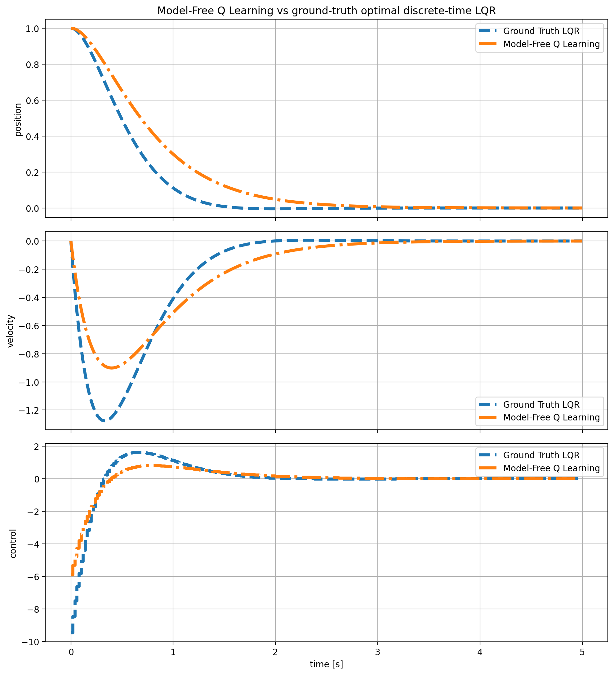
Model-free Q Learning Result.
6. Solving Discounted LQR
So far, the discussion has focused on the standard infinite-horizon discrete-time LQR problem, where future costs are not explicitly discounted. It is also useful to consider a discounted version, especially because many reinforcement-learning formulations are written in that form. Once a discount factor is introduced, however, the underlying optimal control problem changes, and so do the Bellman equation, the optimal feedback law, and the Riccati equation.
Consider the discrete-time linear system
\[x_{k+1}=Ax_k+Bu_k,\]together with the discounted infinite-horizon quadratic cost
\[J_\gamma(x_0,\{u_k\})=\sum_{k=0}^{\infty}\gamma^k\left(x_k^\top Qx_k+u_k^\top Ru_k\right), \qquad 0<\gamma<1.\]Here, \(Q\succeq 0\) penalizes the state, \(R\succ 0\) penalizes the control input, and the discount factor \(\gamma\) reduces the weight assigned to costs further in the future. When \(\gamma<1\), this is no longer the standard undiscounted LQR problem; it is a discounted optimal control problem.
The Bellman optimality equation for this problem is
\[V^*(x)=\min_u\left[x^\top Qx+u^\top Ru+\gamma V^*(Ax+Bu)\right].\]As in the usual LQR derivation, assume that the optimal value function is quadratic:
\[V^*(x)=x^\top Px,\]for some symmetric matrix \(P\). Substituting this ansatz into the Bellman equation yields
\[x^\top Px = \min_u \left[ x^\top Qx+u^\top Ru+\gamma(Ax+Bu)^\top P(Ax+Bu) \right].\]The next step is to derive the minimizing control law explicitly. Expand the quadratic term:
\[(Ax+Bu)^\top P(Ax+Bu) = x^\top A^\top PAx + x^\top A^\top PBu + u^\top B^\top PAx + u^\top B^\top PBu.\]Since the two middle terms are scalars, they are equal:
\[x^\top A^\top PBu = u^\top B^\top PAx.\]Therefore,
\[(Ax+Bu)^\top P(Ax+Bu) = x^\top A^\top PAx + 2u^\top B^\top PAx + u^\top B^\top PBu.\]Substituting this into the Bellman expression gives
\[x^\top Px = \min_u \left[ x^\top Qx + u^\top Ru + \gamma x^\top A^\top PAx + 2\gamma u^\top B^\top PAx + \gamma u^\top B^\top PBu \right].\]To minimize with respect to \(u\), differentiate the right-hand side with respect to \(u\). The terms \(x^\top Qx\) and \(\gamma x^\top A^\top PAx\) do not depend on \(u\), so their derivatives are zero. For the remaining terms, use standard quadratic identities:
\[\frac{\partial}{\partial u}(u^\top Ru)=2Ru,\] \[\frac{\partial}{\partial u}\left(2\gamma u^\top B^\top PAx\right)=2\gamma B^\top PAx,\]and, since \(B^\top PB\) is symmetric,
\[\frac{\partial}{\partial u}\left(\gamma u^\top B^\top PBu\right)=2\gamma B^\top PBu.\]Hence the first-order optimality condition is
\[2Ru+2\gamma B^\top PBu+2\gamma B^\top PAx=0.\]Dividing by \(2\) gives
\[Ru+\gamma B^\top PBu+\gamma B^\top PAx=0,\]which can be rearranged as
\[(R+\gamma B^\top PB)u=-\gamma B^\top PAx.\]This is exactly the linear equation that determines the minimizing control. Assuming \(R+\gamma B^\top PB\) is invertible, the optimal control law is
\[u^*=-Kx,\]with feedback gain
\[\begin{array}{|c|} \hline \displaystyle K=(R+\gamma B^\top PB)^{-1}(\gamma B^\top PA). \\ \hline \end{array}\]This is the discounted analogue of the usual LQR feedback law. Compared with the undiscounted case, the factor \(\gamma\) appears both in the gain numerator and inside the matrix multiplying \(u\). Intuitively, because future costs are discounted, the controller is optimizing a different tradeoff between immediate effort and future state regulation.
To obtain the Riccati equation, substitute this minimizing control back into the Bellman equation. Starting from
\[x^\top Px = x^\top Qx+u^\top Ru+\gamma(Ax+Bu)^\top P(Ax+Bu),\]expand the last term:
\[\gamma(Ax+Bu)^\top P(Ax+Bu) = \gamma x^\top A^\top PAx + 2\gamma u^\top B^\top PAx + \gamma u^\top B^\top PBu.\]Therefore,
\[x^\top Px = x^\top Qx + \gamma x^\top A^\top PAx + u^\top Ru + 2\gamma u^\top B^\top PAx + \gamma u^\top B^\top PBu.\]Now substitute
\[u=-(R+\gamma B^\top PB)^{-1}(\gamma B^\top PA)x.\]Rather than expanding every term separately from scratch, it is cleaner to use the first-order condition
\[(R+\gamma B^\top PB)u=-\gamma B^\top PAx.\]Premultiplying by \(u^\top\) gives
\[u^\top(R+\gamma B^\top PB)u=-\gamma u^\top B^\top PAx.\]Equivalently,
\[u^\top Ru+\gamma u^\top B^\top PBu=-\gamma u^\top B^\top PAx.\]Substitute this identity into the Bellman expression:
\[x^\top Px = x^\top Qx + \gamma x^\top A^\top PAx + \gamma u^\top B^\top PAx.\]Now replace \(u\) by the minimizing control:
\[\gamma u^\top B^\top PAx = -\gamma^2 x^\top A^\top PB(R+\gamma B^\top PB)^{-1}B^\top PAx.\]Hence
\[x^\top Px = x^\top Qx + \gamma x^\top A^\top PAx - \gamma^2 x^\top A^\top PB(R+\gamma B^\top PB)^{-1}B^\top PAx.\]Since this identity holds for all \(x\), the corresponding quadratic forms must be equal, yielding the discounted discrete-time algebraic Riccati equation
\[\begin{array}{|c|} \hline \displaystyle P = Q+\gamma A^\top PA - \gamma^2 A^\top PB(R+\gamma B^\top PB)^{-1}B^\top PA. \\ \hline \end{array}\]This is the correct Riccati equation for discounted LQR. It reduces to the standard undiscounted ARE when \(\gamma=1\). The effect of discounting is systematic: the future-value term introduces one factor of \(\gamma\), while the substitution of the minimizing control introduces a second factor, producing the \(\gamma^2\) term in the nonlinear part of the equation.
It is also useful to interpret this result from a computational perspective. The matrix \(P\) still characterizes the optimal quadratic value function, and the optimal control remains linear in the state, but both are now associated with the discounted objective. Thus, if one solves the discounted Riccati equation, the resulting feedback gain is optimal for the discounted problem, not for the standard undiscounted LQR problem.
A convenient way to view the discounted ARE is through a scaled system. If one defines
\[\begin{array}{|c|} \hline \displaystyle \bar A=\sqrt{\gamma}\,A, \qquad \bar B=\sqrt{\gamma}\,B, \\ \hline \end{array}\]then the discounted Riccati equation becomes the standard undiscounted ARE for the pair \((\bar A,\bar B)\):
\[P = Q+\bar A^\top P\bar A - \bar A^\top P\bar B(R+\bar B^\top P\bar B)^{-1}\bar B^\top P\bar A.\]This observation is often useful in practice, since it allows the discounted problem to be solved using standard discrete-time ARE routines after scaling the dynamics appropriately.
In summary, the discounted LQR problem modifies the standard infinite-horizon quadratic regulation problem by weighting future costs with a factor \(\gamma^k\). This changes the Bellman equation, the optimal linear feedback law, and the Riccati equation. The optimal policy is still of the form \(u_k=-Kx_k\), but the gain now satisfies
\[\begin{array}{|c|} \hline \displaystyle K=(R+\gamma B^\top PB)^{-1}(\gamma B^\top PA), \\ \hline \end{array}\]where \(P\) solves the discounted discrete-time ARE
\[\begin{array}{|c|} \hline \displaystyle P = Q+\gamma A^\top PA - \gamma^2 A^\top PB(R+\gamma B^\top PB)^{-1}B^\top PA. \\ \hline \end{array}\]These equations will form the basis for the policy-iteration and value-iteration algorithms for discounted LQR in the next subsections.
6.1 Policy Iteration
The discounted version of policy iteration has exactly the same structure as in standard LQR: a policy-evaluation step followed by a policy-improvement step. The only change is that future cost terms are multiplied by \(\gamma\).
For a fixed feedback law
\[u_k^j=-K^j x_k,\]the value function is again taken as quadratic,
\[V^j(x)=x^\top P^j x.\]Substituting this into the discounted Bellman equation gives the discounted policy-evaluation equation
\[\begin{array}{|c|} \hline \displaystyle P^j = Q+(K^j)^\top R K^j+\gamma (A-BK^j)^\top P^j (A-BK^j). \\ \hline \end{array}\]So this is just the standard Lyapunov equation with an extra factor \(\gamma\) in front of the closed-loop term.
That is exactly why the SciPy call changes in a simple way. If
\[A_{\mathrm{cl}}=A-BK^j,\]then the discounted equation can be rewritten as
\[\begin{array}{|c|} \hline \displaystyle P^j = Q+(K^j)^\top R K^j + (\sqrt{\gamma}A_{\mathrm{cl}})^\top P^j (\sqrt{\gamma}A_{\mathrm{cl}}). \\ \hline \end{array}\]So, instead of passing the undiscounted closed-loop matrix to
\[\sqrt{\gamma}(A-BK^j).\]solve_discrete_lyapunov, you pass the scaled one:In code terms, the argument changes from the usual closed-loop matrix to its \(\sqrt{\gamma}\)-scaled version, while the right-hand-side term remains
\[Q+(K^j)^\top R K^j.\]The policy-improvement step also has the same form as before, except that \(\gamma\) appears inside the gain formula:
\[K^{j+1}=(R+\gamma B^\top P^j B)^{-1}(\gamma B^\top P^j A).\]So, relative to standard LQR, discounted policy iteration is obtained by replacing:
- the Lyapunov equation with its discounted version,
- the gain update with the discounted gain formula.
In short, discounted policy iteration is the standard algorithm with a systematic \(\gamma\)-modification in both evaluation and improvement.
6.2 Value Iteration
The discounted version of value iteration is obtained by applying the discounted Bellman optimality operator directly to the quadratic value function. If
\[V^j(x)=x^\top P^j x,\]then the next iterate is
\[\begin{array}{|c|} \hline \displaystyle P^{j+1} = Q+\gamma A^\top P^j A - \gamma^2 A^\top P^j B (R+\gamma B^\top P^j B)^{-1} B^\top P^j A. \\ \hline \end{array}\]This is the discounted Riccati recursion. It is the direct analogue of the standard value-iteration update, with \(\gamma\) appearing in the future-value term and \(\gamma^2\) in the nonlinear term.
Once \(P^{j+1}\) is updated, the greedy controller is read out as
\[\begin{array}{|c|} \hline \displaystyle K^{j+1} = (R+\gamma B^\top P^{j+1} B)^{-1} (\gamma B^\top P^{j+1} A).\\ \hline \end{array}\]For the ground-truth discounted optimal solution, the SciPy
\[P = Q+\gamma A^\top P A - \gamma^2 A^\top P B (R+\gamma B^\top P B)^{-1} B^\top P A\]solve_discrete_arecall also changes by the same scaling trick used in Section 6. The discounted AREis equivalent to the standard ARE for the scaled pair
\[\bar A=\sqrt{\gamma}\,A, \qquad \bar B=\sqrt{\gamma}\,B.\]So, instead of calling
\[\texttt{solve_discrete_are}(\sqrt{\gamma}A,\sqrt{\gamma}B,Q,R).\]solve_discrete_are(A, B, Q, R), you callThat is the main practical takeaway:
- for
solve_discrete_are, replace \(A,B\) by \(\sqrt{\gamma}A,\sqrt{\gamma}B\); - for
solve_discrete_lyapunov, replace the closed-loop matrix \(A-BK\) by \(\sqrt{\gamma}(A-BK)\).
So the discounted case does not require a new solver. It uses the standard ARE and Lyapunov solvers, but with appropriately scaled dynamics.
- for
6.3 Model-free Q Learning and Results
For model-free Q learning, the procedures are pretty much the same as illustrated in section 5.3, except with an addition discount factor \(\gamma\). The results for all three methods are shown as follows:
Policy Iteration Result (discounted). Value Iteration Result (discounted). Model-free Q Learning Result (discounted).
7. Correspondence to Pontryagin’s Minimum Principle
The dynamic-programming viewpoint and Pontryagin’s Minimum Principle (PMP) are often presented as two different routes to optimal control. In fact, they are closely related. Dynamic programming starts from the value function and Bellman’s equation, while PMP starts from constrained trajectory optimization and introduces the co-state as a Lagrange multiplier for the dynamics. For the same optimal control problem, both approaches lead to the same optimality conditions, but they express them in different variables.
For the discrete-time LQR problem considered in this post, this correspondence is especially transparent. The value function is quadratic, the co-state is linear in the state, and the resulting optimal controller is linear. Thus, the Bellman/HJB and PMP viewpoints are not competing descriptions; rather, they are two different ways of encoding the same optimality structure.
7.1 Hamiltonian Formulation
In PMP, the Hamiltonian is written explicitly in terms of the state, control, and co-state. For a discrete-time system of the form
\[x_{k+1}=f(x_k,u_k),\]with stage cost
\[\ell(x_k,u_k),\]the PMP Hamiltonian is typically written as
\[\mathcal{H}(x_k,u_k,\lambda_{k+1}) = \ell(x_k,u_k)+\lambda_{k+1}^\top f(x_k,u_k).\]The control action is then chosen to minimize this Hamiltonian with respect to \(u_k\).
By contrast, in the Bellman / HJB viewpoint, one starts from the expression inside Bellman’s minimization. In discrete time, the Bellman optimality equation is
\[V(x_k)=\min_{u_k}\bigl[\ell(x_k,u_k)+V(x_{k+1})\bigr], \qquad x_{k+1}=f(x_k,u_k),\]or, with discounting,
\[V(x_k)=\min_{u_k}\bigl[\ell(x_k,u_k)+\gamma V(x_{k+1})\bigr].\]If one defines the Bellman expression
\[\mathcal{J}(x_k,u_k):=\ell(x_k,u_k)+V(x_{k+1}),\]or in the discounted case
\[\mathcal{J}(x_k,u_k):=\ell(x_k,u_k)+\gamma V(x_{k+1}),\]then the optimal control satisfies the stationarity condition
\[\frac{\partial \mathcal{J}}{\partial u_k}=0.\]This is the HJB stationarity condition.
A closely related quantity is the Bellman residual
\[\begin{array}{|c|} \hline \displaystyle \ell(x_k,u_k)+V(x_{k+1})-V(x_k), \\ \hline \end{array}\]or, in the discounted case,
\[\ell(x_k,u_k)+\gamma V(x_{k+1})-V(x_k).\]This residual measures whether the Bellman equation is satisfied at the current state-action pair. If one chooses to call this residual a Bellman-style “Hamiltonian,” then minimizing it with respect to \(u_k\) is equivalent to minimizing
\[\ell(x_k,u_k)+V(x_{k+1}),\]because the term \(V(x_k)\) does not depend on the control . In that sense, the Bellman-residual Hamiltonian and the Bellman expression lead to the same stationarity condition.
This is exactly where the bridge to PMP appears. Differentiating the Bellman expression with respect to \(u_k\) gives
\[\frac{\partial \ell(x_k,u_k)}{\partial u_k} + \frac{\partial V(x_{k+1})}{\partial u_k} =0.\]Applying the chain rule to the value term yields
\[\frac{\partial V(x_{k+1})}{\partial u_k} = \bigl(\nabla_x V(x_{k+1})\bigr)^\top \frac{\partial x_{k+1}}{\partial u_k} = \bigl(\nabla_x V(x_{k+1})\bigr)^\top \frac{\partial f(x_k,u_k)}{\partial u_k}.\]Hence the first-order condition becomes
\[\begin{array}{|c|} \hline \displaystyle \frac{\partial \ell(x_k,u_k)}{\partial u_k} + \bigl(\nabla_x V(x_{k+1})\bigr)^\top \frac{\partial f(x_k,u_k)}{\partial u_k} =0, \\ \hline \end{array}\]or, in the discounted case,
\[\begin{array}{|c|} \hline \displaystyle \frac{\partial \ell(x_k,u_k)}{\partial u_k} + \gamma \bigl(\nabla_x V(x_{k+1})\bigr)^\top \frac{\partial f(x_k,u_k)}{\partial u_k} =0. \\ \hline \end{array}\]This has exactly the PMP form once the co-state is identified with the gradient of the value function . Thus, the PMP Hamiltonian can be viewed as the first-order, co-state-based form of the HJB/Bellman expression.
7.2 Co-state and Value Function
The key link between PMP and dynamic programming is the relation between the co-state and the gradient of the value function. In PMP, the co-state measures the sensitivity of the total cost with respect to the state. In dynamic programming, that same sensitivity is represented by the gradient of the cost-to-go. Therefore, under suitable smoothness assumptions, along an optimal trajectory one has
\[\begin{array}{|c|} \hline \displaystyle \lambda_k = \nabla_x V^*(x_k), \qquad\text{or equivalently in discrete time}\qquad \lambda_{k+1}=\nabla_x V^*(x_{k+1}), \\ \hline \end{array}\]depending on the indexing convention.
This is the standard PMP–HJB correspondence, and it is tied to optimality. It is important not to overstate it. The identity above does not mean that the co-state along an arbitrary nonoptimal trajectory is always the gradient of the optimal value function. That would generally be false, because \(V^*\) encodes the cost-to-go under optimal future decisions, while a nonoptimal trajectory is generated by a different control law.
A more precise statement is the following. If one fixes an arbitrary admissible policy \(\pi\), then one can define its policy-specific value function
\[V^\pi(x).\]Along a trajectory generated by that policy, the analogous sensitivity relation is
\[\begin{array}{|c|} \hline \displaystyle \lambda_k^\pi = \nabla_x V^\pi(x_k). \\ \hline \end{array}\]So a gradient-to-co-state relation also exists for nonoptimal trajectories, provided one is talking about the value function associated with the same policy that generates that trajectory . Thus:
- along an optimal trajectory, the co-state equals the gradient of the optimal value function;
- along a fixed nonoptimal policy, the corresponding co-state-like sensitivity equals the gradient of that policy’s own value function \(V^\pi\);
- one should not identify the co-state of an arbitrary nonoptimal trajectory with \(\nabla_x V^*\) unless that trajectory is actually optimal.
In the LQR setting, this relation becomes especially simple. Throughout this post, the value function has been written with the \(1/2\) convention:
\[V(x_k)=\frac{1}{2}x_k^\top P x_k.\]With this normalization, and using the symmetry of \(P\), its gradient is
\[\nabla_x V(x_k)=P x_k.\]This is precisely why the \(1/2\) convention is convenient: it removes the extra factor of \(2\) from the gradient. Therefore, in discrete-time LQR, the co-state is linear in the state:
\[\lambda_k = P x_k.\]This makes the correspondence fully explicit. The value function is quadratic, its gradient is linear, and so the co-state is linear as well. The stationarity condition in PMP can therefore be written directly in terms of \(P x_k\), which is the same matrix quantity that appears in the Riccati equation and in the Bellman derivation of the optimal controller.
The same connection can also be read directly from the Bellman-residual viewpoint. Since
\[\frac{\partial V(x_{k+1})}{\partial u_k} = \bigl(\nabla_x V(x_{k+1})\bigr)^\top \frac{\partial x_{k+1}}{\partial u_k},\]the derivative of the Bellman expression already contains the PMP-style co-state term, but written through the value function gradient. Thus, the co-state does not need to be introduced separately in the Bellman viewpoint; it is already present implicitly through the dependence of the next-state value on the control.
For LQR, this means that the same matrix \(P\) plays several roles simultaneously:
- it defines the quadratic value function,
- it determines the co-state through \(\lambda_k=P x_k\),
- and it determines the optimal feedback law through the Riccati equation.
This is why the Bellman/HJB and PMP approaches ultimately give the same controller. One expresses optimality through the value function and Bellman recursion, while the other expresses it through the co-state and Hamiltonian minimization. In the linear-quadratic setting, the two viewpoints meet exactly through the identity between the co-state and the gradient of the value function.
8. Solving Discounted LQR Using Only the Input Matrix \(g(x)\)
The fully model-based discounted LQR algorithms in the previous sections assume knowledge of both system matrices \(A\) and \(B\). At the other extreme, the Q-learning approach avoids using either matrix explicitly by learning a state-action value function directly from data. Between these two lies an intermediate setting: the control designer may know only the input matrix \(g(x)\), or \(B\) in the linear case, while the rest of the system dynamics remain unknown. This leads to a partially model-based approach that still uses Bellman equations, but performs policy improvement through the known input channel rather than through a learned Q function.
The key observation is that Bellman’s equation for the value function does not by itself require a full analytical model when used in sample-based form. If one can observe transitions \(x_k \mapsto x_{k+1}\) and evaluate the one-step cost, then the value function can be learned from trajectory data . What the known input matrix \(B\) provides is a way to convert the learned value function into an improved control law. Thus, this approach is Bellman-based and data-driven on the critic side, but analytically structured on the policy-improvement side.
For the discounted problem, consider dynamics of the form
\[x_{k+1}=f(x_k)+g(x_k)u_k,\]with stage cost
\[\ell(x_k,u_k)=Q(x_k)+u_k^\top R u_k,\]and Bellman equation
\[V(x_k)=\min_{u_k}\bigl[\ell(x_k,u_k)+\gamma V(x_{k+1})\bigr].\]Differentiating the expression inside the Bellman minimization with respect to \(u_k\) gives
\[\frac{\partial \ell(x_k,u_k)}{\partial u_k} + \gamma \bigl(\nabla_x V(x_{k+1})\bigr)^\top \frac{\partial x_{k+1}}{\partial u_k} =0.\]Since
\[x_{k+1}=f(x_k)+g(x_k)u_k,\]one has
\[\frac{\partial x_{k+1}}{\partial u_k}=g(x_k).\]With the quadratic control cost, \(\partial \ell / \partial u_k = 2Ru_k\), so the optimality condition becomes
\[2Ru_k+\gamma g^\top(x_k)\nabla_x V(x_{k+1})=0.\]Therefore, the policy-improvement formula is
\[\begin{array}{|c|} \hline \displaystyle u_k^*=-\frac{\gamma}{2}R^{-1}g^\top(x_k)\nabla_x V(x_{k+1}). \\ \hline \end{array}\]In the discrete-time LQR case, \(g(x)=B\), so this reduces to
\[u_k^*=-\frac{\gamma}{2}R^{-1}B^\top \nabla_x V(x_{k+1}).\]This formula is the defining feature of the \(B\)-only method. It says that once a value function has been learned, the next control can be improved using only the gradient of that value function and the known input matrix \(B\). Full knowledge of \(A\) is not needed for the policy-improvement step. Instead, the unknown part of the dynamics is handled implicitly through observed state transitions, while the known input structure is used explicitly to compute the control update.
It is also useful to connect this formula to the PMP correspondence. In the discounted setting, one may define the co-state as
\[\lambda_{k+1}=\nabla_x V(x_{k+1}),\]in which case the stationarity condition reads
\[\begin{array}{|c|} \hline \displaystyle \frac{\partial \ell}{\partial u_k} + \gamma \lambda_{k+1}^\top \frac{\partial f}{\partial u_k} =0. \\ \hline \end{array}\]Alternatively, one may absorb the discount factor into the co-state and define
\[\lambda_{k+1}=\gamma \nabla_x V(x_{k+1}),\]so that the stationarity condition takes the more standard PMP-looking form
\[\frac{\partial \ell}{\partial u_k} + \lambda_{k+1}^\top \frac{\partial f}{\partial u_k} =0.\]Both conventions are valid. The difference is only whether the factor \(\gamma\) is written explicitly in the stationarity condition or absorbed into the definition of the co-state. In either case, the policy-improvement formula above is exactly the Bellman/HJB stationarity condition rewritten in a PMP-like form.
8.1 Policy Iteration
In the \(B\)-only version of policy iteration, the current policy is first evaluated from sampled data, and then improved analytically using the known input matrix.
Suppose a policy \(\pi_j(x_k)\) is fixed at iteration \(j\). Instead of solving a model-based Lyapunov equation, one fits a critic \(V_{j+1}(x)\) so that the Bellman equation for that policy is approximately satisfied along the observed rollout:
\[V_{\color{red}{j+1}}(x_k)\approx r(x_k,\pi_j(x_k))+\gamma V_{\color{red}{j+1}}(x_{k+1}).\]In the paper, this fitting step is expressed using a linear parameterization and solved by least squares or RLS. The essential idea, however, is simply policy evaluation from data: the value function is adjusted so that it becomes consistent with the one-step Bellman recursion under the current controller .
If one does not use RLS, this step can be viewed as a regression problem against a Bellman target. Suppose the critic is parameterized by \(\theta\), so that the value estimate is \(V_\theta(x)\). Then for each observed transition one forms the target
\[y_k = r(x_k,\pi_j(x_k))+\gamma V_{\bar\theta}(x_{k+1}),\]where \(V_{\bar\theta}\) may be the current critic, a frozen previous iterate, or a target network. One then minimizes a loss such as
\[\mathcal{L}(\theta)=\sum_k \bigl(V_\theta(x_k)-y_k\bigr)^2.\]Thus, replacing RLS by gradient descent does not change the Bellman logic. It only changes how the critic parameters are fitted. In both cases, the critic is being trained so that the Bellman equation is satisfied as accurately as possible on the sampled transitions. So yes, it is natural to view this as a regression problem: the critic is regressed toward Bellman-consistent targets.
Once the value estimate has converged sufficiently, the policy is improved using the gradient-based formula
\[\begin{array}{|c|} \hline \displaystyle \pi_{j+1}(x_k)=-\frac{\gamma}{2}R^{-1}g^\top(x_k)\nabla_x V_{j+1}(x_{k+1}). \\ \hline \end{array}\]Thus, policy iteration in this setting still alternates between policy evaluation and policy improvement, but the evaluation is data-driven and the improvement uses only \(g(x)\), or \(B\) in LQR.
For linear quadratic problems, this becomes especially simple. If the value function is parameterized as
\[V_j(x_k)=\frac{1}{2}x_k^\top P_j x_k,\]then
\[\nabla_x V_j(x_k)=P_j x_k,\]and so the policy-improvement step becomes
\[u_k^{j+1}=-\frac{\gamma}{2}R^{-1}B^\top P_{j+1}x_{k+1}.\]Depending on notation and indexing, this may be expressed at the next state or shifted back to the current state through the dynamics. The important point is that the update depends on the learned value matrix \(P_{j+1}\) and the known matrix \(B\), but not on an explicit model for the full state transition map.
8.2 Value Iteration
A similar idea applies to value iteration. Instead of more fully evaluating a fixed policy, one directly updates the value estimate from sampled Bellman recursions. The value-update step takes the form
\[V_{\color{red}{j+1}}(x_k)\approx r(x_k,\pi_j(x_k))+\gamma V_{\color{red}{j}}(x_{k+1}),\]where the next-state value is taken from the previous iterate rather than from a more converged policy-evaluation solve.
As in the policy-iteration case, this update can be implemented either by linear least squares / RLS or by gradient descent on a Bellman residual loss. If \(V_\theta(x)\) is the critic, then one can minimize
\[\mathcal{L}(\theta)=\sum_k \bigl(V_\theta(x_k)-[r_k+\gamma V_{\bar\theta}(x_{k+1})]\bigr)^2\]over rollout data. Again, the interpretation is the same: the critic is being trained so that the Bellman equation is approximately satisfied over the encountered states and transitions.
Once the updated value function \(V_{j+1}\) is obtained, the control policy is improved using the same formula as before:
\[\pi_{j+1}(x_k)=-\frac{\gamma}{2}R^{-1}g^\top(x_k)\nabla_x V_{j+1}(x_{k+1}).\]Thus, the difference between the policy-iteration and value-iteration variants lies in how the critic is updated:
- in policy iteration, the value function is first fit to the Bellman equation of the current policy more completely ;
- in value iteration, only a one-step Bellman update is used before improving the policy .
The policy-improvement step is the same in both cases. In that sense, the \(B\)-only method inherits exactly the same distinction between policy iteration and value iteration that appeared earlier in the fully model-based setting. The only difference is that the value update is now driven by sampled data rather than by a known system model.
8.3 Compare with Model-free Q Learning
Compared with the fully model-based approach, it uses less model information. It does not require complete knowledge of the state transition dynamics, so the critic can be learned from data rather than computed from a Riccati or Lyapunov equation. This makes it more flexible when the full system model is unavailable.
Compared with Q-learning, however, it still uses structural knowledge through the input matrix \(B\). That extra knowledge is important, because it allows policy improvement to be written directly in terms of the value-function gradient. As a result, the critic only needs to approximate a value function \(V(x)\), rather than a full state-action function \(Q(x,u)\). For LQR, this means learning a quadratic matrix \(P\) rather than a larger quadratic kernel \(S\) over \((x,u)\). Since the value-based object is smaller, this approach can be more structured and potentially more sample efficient than a fully model-free Q-function method.
The tradeoff is therefore clear:
- fully model-based LQR uses \(A\) and \(B\), and computes the solution analytically;
- the \(B\)-only method learns the value function from data, but uses \(B\) to improve the policy;
- model-free Q-learning learns a full state-action critic and does not require either \(A\) or \(B\).
From the Bellman perspective, both the \(B\)-only method and the Q-learning method are based on exactly the same principle: the critic is updated so that Bellman consistency is enforced on sampled transitions . The difference is what the critic represents and how policy improvement is carried out afterward. In the \(B\)-only method, the critic is \(V(x)\), and policy improvement uses the known input matrix together with the gradient of the value function. In the Q-learning method, the critic is \(Q(x,u)\), and policy improvement is performed by directly minimizing the learned state-action cost.
In that sense, the \(B\)-only method is a particularly interesting middle ground. It preserves part of the control-theoretic structure of LQR through the known input matrix, while still allowing the critic to be learned from trajectory data. That makes it a natural bridge between classical model-based control and fully model-free reinforcement learning.