
On Derivation of Euluer-Lagrange Equation and Its Application
Published:
Euler-Lagrange equation plays an essential role in calculus of variations and classical mechanics. Beyond its applications in deriving equations of motion, Euler-Lagrange equation is ubiquitous in the filed of trajectory optimization, serving as a critical stepping stone for many powerful optimal control techniques, such as Pontrygain’s Maximum Principle. In this blog, derivation of the Euler-Lagrange equation and two simple cases of its application are introduced.
Derivation of Euler-Lagrange Equation
Similar to finding the maximum or minimum of a function, which requires finding the points such that function has zero derivate, the extremal of a functional requries finding the functions that make corresponding functional dertivate equal to 0. Let’s define the objective functional \(J\) that takes \(q(t)\), \(\dot{q}(t)\) and \(t\) as the argument, where \(q(t)\) represent generatlized coordinates (i.e. Cartisian, Polar, etc.) and \(\dot{q}(t)\) represents the derivative of \(q(t)\).
\[J[q] = \int_{t_1}^{t_2} L(q(t), \dot{q}(t), t) \, dt \\\]For the seek of concise notation, I will denote \(q(t)\) as \(q\) and \(\dot{q}(t)\) as \(\dot{q}\) in the later section, but keep in mind that they are both functions of time. Note that here we are considering the case with fixed initial and final states and a fixed time interval from \(t_1\) to \(t_2\). Thus, for a optimal functional \( J^* \), its functional derivative \(\frac{\delta J}{\delta q}\) should be zero. In other word, if we perturb its arguments \( q^* \) and \(q(t)^* \), the corresponding \(\delta J\) should also be zero. This means that a small perturbation of \( q^* \) does not produce a first-order change (first variation) in \(J[q]\).
Suppose we perturb \( q^* \) by \(\delta q \) and \(\dot{q}^* \) by \(\delta \dot{q}\) respectively, then based on the law of total derivatives:
\[\delta J^* = \int_{t_1}^{t_2} \left( \frac{\partial L}{\partial q} \cdot \delta q + \frac{\partial L}{\partial \dot{q}} \cdot \delta \dot{q} \right) dt = 0\]Since \(\delta \dot{q} \) is the derivative of \(\delta q\), we can express \(\delta \dot{q} \) in the form of \(\delta q\) through integration by part:
\[\frac{\partial L}{\partial \dot{q}} \cdot \delta \dot{q} = \frac{d}{dt} \left( \frac{\partial L}{\partial \dot{\vec{q}}} \right) \cdot \delta q \, + \cancelto{}{\left[ \frac{\partial L}{\partial \dot{\vec{q}}} \cdot \delta \vec{q} \right]_{t_1}^{t_2}}\]Noticed that since both initial state and final state are fixed, and we are dealing with optimization over a fixed time interval, the variation of \(\delta q\) should be zero at both time \(t_1\) and \(t_2\). (\(\delta q(t_1) = \delta q(t_2) = 0\)). Therefore, the second term in the above expression vanishes and \(\delta J^*\) can be expressed as follows:
\[\delta J[q]^* = \int_{t_1}^{t_2} \left( \frac{\partial L}{\partial q} - \frac{d}{dt} \left( \frac{\partial L}{\partial \dot{q}} \right) \right) \delta q \, dt = 0\]Since \(\delta q\) can be arbitrary, in order to guarantee \(\delta J^* = 0\), the following condition (Euler-Lagrange Equation) needs to be held:
\[\frac{\partial L}{\partial q} - \frac{d}{dt} \left( \frac{\partial L}{\partial \dot{q}} \right) = 0\]In short, Euler-Lagrange Equation provides first-order necessary conditions (FONC) for a differentiable functional to have an extremum on some function. In order to determine whether the candidate solution is a minimum or maximum, Legendre–Clebsch condition needs to be used, which is similar to the use of Hessian for regular functions.
Euler-Lagrange Equation with Constraints
Let’s consider the case where there exists holonomic constraints in the dynamical system.
\[f(q,t) = 0\, \quad \forall \, q \quad \rightarrow \quad \delta f = \frac{\partial f}{\partial q} \cdot \delta q = 0\]In this case, \(\delta q\) can not be arbitrary because constraint needs to be satisfied. Since \(\delta f(\delta q, t) = 0\), we can mulitply it with Lagrange multipliers \(\lambda\) and add it into the integration but still keep the result (\(J[q]\)) unchanged.
\[\delta J[q]^* = \int_{t_1}^{t_2} \left( \frac{\partial L}{\partial q} - \frac{d}{dt} \left( \frac{\partial L}{\partial \dot{q}} \right) + \lambda \frac{\partial f}{\partial q} \right) \delta q \, dt = 0\]Therefore, the conditions becomes as follows for a stationary point of the functional \(J[q]\)
\[\frac{\partial L}{\partial q} - \frac{d}{dt} \left( \frac{\partial L}{\partial \dot{q}} \right) + \lambda \frac{\partial f}{\partial q} = 0 \quad \& \quad f(q,t) = 0\]Example 1: Get equations of motion for a pendulum.
The Euler-Lagrange Equation is a fundamental component of Lagrangian Mechanics, providing a powerful framework for deriving the equations of motion for various systems. Lagrangian Mechanics is convenient when dealing with forces of constraint and generalized coordinates, as it allows for a more straightforward analysis of these systems.
Lagrangian Mechanics offers several advantages over Newtonian Mechanics, particularly in its ability to handle more sophisticated systems such as the acrobot (underactuated double pendulum). This approach simplifies the process of obtaining equations of motion by focusing on energy principles rather than forces, making it especially useful for systems with constraints or those that involve complex interactions. Here, we just use the simple pendulum for illustration.
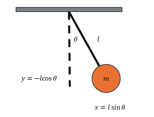
Let’s consider a massless rod with length \(l\) and a ball with mass of \(m kg\) attacehd at the end of rod. The Lagrangian is defined as the sum of potential engery \(U\) and kinetic energy \(T\), which are shown as follows:
\[U = mgy = -mgl \cos \theta, \quad T = \frac{1}{2}m(\dot{x}^2 + \dot{y}^2)\]After converting \(x\) to \(\theta\) use the relations as shown in the picture, the kinetic energy \(T\) can be rewritten as:
\[\dot{x} = \frac{d}{dt}(l \sin \theta) = l \cos \theta \dot{\theta}, \quad \dot{y} = \frac{d}{dt}(l \cos \theta) = -l \sin \theta \dot{\theta}\] \[T = \frac{1}{2}m(l^2 \cos^2 \theta \dot{\theta}^2 + l^2 \sin^2 \theta \dot{\theta}^2) = \frac{1}{2}ml^2 \dot{\theta}^2\]Thus the Lagrangian of this simple pendulum system is:
\[L = T - U = \frac{1}{2}ml^2 \dot{\theta}^2 + mgl \cos \theta\]Taking the necessary partial derivatives of Lagrangian,
\[\frac{\partial L}{\partial \theta} = -mgl \sin \theta, \quad \frac{\partial L}{\partial \dot{\theta}} = ml^2 \dot{\theta},\quad \frac{d}{dt} \frac{\partial L}{\partial \dot{\theta}} = ml^2 \ddot{\theta}\]then substitute into Euler-Lagrange Equation,
\[\frac{\partial L}{\partial \theta} - \frac{d}{dt} \frac{\partial L}{\partial \dot{\theta}} = 0\]we obtained the final equations of motion, which is the same result using Newtonoian approach.
\[-mgl \sin \theta - ml^2 \ddot{\theta} = 0\]After simplifyingt the expression, the dynamics of this simple pendulum can be expressed as
\[\ddot{\theta} = -\frac{g}{l} \sin \theta, \quad or \quad \begin{bmatrix} \dot{\theta} \\ \ddot{\theta} \end{bmatrix} = \begin{bmatrix} 0 & 1 \\ -\frac{g \sin \theta}{l} & 0 \end{bmatrix} \begin{bmatrix} \theta \\ \dot{\theta} \end{bmatrix}.\]Example 2: Solving a simple trajectory optimzation problem
Consider the following simple robot dynamics (single-integrator model) and the objetive functional aimed to minimize:
\[J = \frac{1}{2} \int_{0}^{1} (x^2 + u^2) \, dt\] \[s.t. x(0) = 0, x(1) = 10, \dot{x} = u(t)\]Step 1: Set up the functional
Since the control input directly impact on the robot’s velocity, the objective functional and its corresponding Lagrangian can be expressed as:
\[J[x] = \frac{1}{2} \int_{0}^{1} (x^2 + \dot{x}^2) \, dt\] \[L(x, \dot{x}, t) = \frac{1}{2} (x^2 + \dot{x}^2)\]Step 2: Apply the Euler-Lagrange equation
First, compute necessary partial derivatives and time derivative:
\[\frac{\partial L}{\partial x} = x, \quad \frac{\partial L}{\partial \dot{x}} = \dot{x}\] \[\frac{d}{dt} \left( \frac{\partial L}{\partial \dot{x}} \right) = \frac{d}{dt} (\dot{x}) = \ddot{x}\]Substitute these component into the Euler-Lagrange equation we get:
\[\ddot{x} - x = 0\]Step 3: Solve the differential equation
The differential equation \( \ddot{x} - x = 0 \) is a second-order linear homogeneous differential equation. Its characteristic equation is:
\[r^2 - 1 = 0, \quad r = \pm 1\]Thus, the general solution to the differential equation is:
\[x(t) = Ae^t + Be^{-t}, \quad u(t) = Ae^t - Be^{-t}\]Step 4: Apply the boundary conditions
Use the boundary conditions \( x(0) = 0 \) and \( x(1) = 10 \) to solve for \( A \) and \( B \):
- At \( t = 0 \):
- At \( t = 1 \):
We have the system of equations:
\[A + B = 0\] \[Ae + Be^{-1} = 10\]Thus, solution can be easily derived as follows:
\[A = \frac{10}{e - e^{-1}} \quad B = -\frac{10}{e - e^{-1}}\]Step 5: Write the extremal function
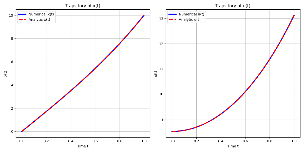
Substitute \( A \) and \( B \) back into the optimal state and control input trajectory:
\[x^*(t) = \frac{10e^t}{e - e^{-1}} - \frac{10e^{-t}}{e - e^{-1}} = \frac{10(e^t - e^{-t})}{e - e^{-1}}\] \[u^*(t) = \dot{x}^*(t) = \frac{10(e^t + e^{-t})}{e - e^{-1}}\]Below is the python code that first solves this two point boundary value problem numerically using solve_bvp function from scipy and compare it with the solution obtained analytically as shown above.
import numpy as np
import matplotlib.pyplot as plt
from scipy.integrate import solve_bvp

# Define the differential equation system
def ode(t, y):
    x, u = y
    dxdt = u
    dudt = x
    return [dxdt, dudt]

# Define the boundary conditions
def bc(ya, yb):
    # ya and yb are the solution vector at t = 0 and tf
    # y[0] = x, y[1] = u
    return [ya[0], yb[0] - 10]

# Initial guess for the solution
t = np.linspace(0, 1, 100)
x_guess = t * 10
# np.gradient -> u = dx/dt
u_guess = np.gradient(x_guess, t)
y_guess = np.vstack((x_guess, u_guess))

# Solve the boundary value problem
sol = solve_bvp(ode, bc, t, y_guess)

# Extract the solution
x_numeric = sol.sol(t)[0]
u_numeric = sol.sol(t)[1]

# Analytical solution
e = np.exp(1)
A = 10 / (e - e**(-1))
B = -A
x_analytic = A * np.exp(t) + B * np.exp(-t)
u_analytic = A * np.exp(t) - B * np.exp(-t)

# Plot the results
plt.figure(figsize=(12, 6))

plt.subplot(1, 2, 1)
plt.plot(t, x_numeric, 'b', label='Numerical x(t)', linewidth = 3)
plt.plot(t, x_analytic, 'r--', label='Analytic x(t)', linewidth = 3)
plt.title('Trajectory of x(t)')
plt.xlabel('Time t')
plt.ylabel('x(t)')
plt.legend()
plt.grid(True)

plt.subplot(1, 2, 2)
plt.plot(t, u_numeric, 'b', label='Numerical u(t)', linewidth = 3)
plt.plot(t, u_analytic, 'r--', label='Analytic u(t)', linewidth = 3)
plt.title('Trajectory of u(t)')
plt.xlabel('Time t')
plt.ylabel('u(t)')
plt.legend()
plt.grid(True)

plt.tight_layout()
plt.show()
Summary
- Euler-Lagrange Equation is essential for functional optimization. Similar to setting the first-order derivatives of a function to be zero for findings its extremum, Euler-Lagrange Equations ensures first variation of a functional to be zero for finding extremals of a functional. This normally results in a system of differential equations and an exact optimal solution (function) can be founded by matching the boundary values.
- Solving Euler-Lagrange Equation is a necessary step in Lagrangian Mechanics, which can have several advantages over Newtonian Mechanics, especially in the case of deriving equations of motions.
- In the second example, \(\dot{x}\) happens to be \(u(t)\) and it is a type of fixed final state and final time unconstrained continuous trajectory optimization problem. To solve for problems with more complex dynamics and other types (i.e. free final state and/or free final time), more conditions needs to be held other than just Euler-Lagrange Equations. It often requires the use of Pontrygain’s Maximum Principle. Typically the optimal solutions are not be able to obtained analytically, and numerical methods are often the choice.
References
- Constrained Lagrangian mechanics: understanding Lagrange multipliers (super excellent and enlightening explanation).
- Introduction to Lagrangian Mechanics (succinct and clear intro with examples).
- Introduction to Variational Calculus - Deriving the Euler-Lagrange Equation (another great explanation on derivation of Euler-Lagrange Equation).
- H.J. Sussmann and J.C. Willems, “300 years of optimal control: from the brachystochrone to the maximum principle,” IEEE Control Systems Magazine, vol. 17, no. 3, pp. 32-44, June 1997.