
From Control Hamiltonian to Algebraic Riccati Equation and Pontryagin’s Maximum Principle
Published:
Inspired by the Hamiltonian of classical mechanics, Lev Pontryagin introduced the Control Hamiltonian and formulated his celebrated Pontragin’s Maximum Principle (PMP). This blog will first discuss general cases of optimal control problems, including scenarios with both free final time and final states. Then, the derivation of Algebraic Riccati Equation (ARE) in the context of Continuous Linear Qudratic Regulator (LQR) from the perspective of the Control Hamiltonian will be introduced. It will then explain the PMP, finally followed by the example problem of Constrained Continous LQR.
More general senarios of trajectory optimization problems
In one of the other blogs on Euler-Lagrange equation, I went through the derivation process for the case of fixed final state and fixed final time. Now, Let’s consider more general cases that involve free final state and free final time. To start with, recall the goal is minimize the objective functional as follows:
\[J[x] = \int_0^{t_f} L(x(t), \dot{x}(t)) \, dt\]The first varition of \(J[x]\) can be written as:
\[\delta J[x] = \int_0^{t_f} \left( \frac{\partial L}{\partial x} \delta x + \frac{\partial L}{\partial \dot{x}} \delta \dot{x} \right) dt\]For the optimal solution, the first varition of the functional \(J[x]\) should be zero. Note that in the later section, for the sake of concise notation, I will use \(L^* \big|_{t_f}\) to denote \(L^*(x(t_f), \dot{x}(t_f))\). Also keep in mind that I will denote \(x(t)\), \(\dot{x}(t)\) as \(x\), \(\dot{x}\) for simplicity too.
Now consider the most general case, where both final state and final time can be free, and the first variation can be expressed as:
\[\delta J[x^*] \approx \int_0^{t_f} \left( \frac{\partial L^*}{\partial x} \delta x + \frac{\partial L^*}{\partial \dot{x}^*} \delta \dot{x} \right) \delta x \, dt + \int_{t_f}^{t_f + \delta t_f} L^* \big|_{t_f} \, dt\]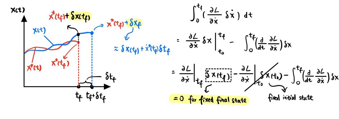
where \(\int_{t_f}^{t_f + \delta t_f} L^* \big|_{t_f} \, dt\) comes from the fact that the final time \(\delta t_f\) is no longer fixed. The reason we can approximate the increment of the objective functional caused by the change of final time as this is that we are doing small perturbation at the optimal \(J[x^*]\). Through integration by part and the fact of fixed initial condition (as shown in the figure above), we can further rearrange the equation as follows:
\[\delta J[x^*] \approx \int_0^{t_f} \left( \frac{\partial L^*}{\partial x^*} - \frac{d}{dt} \frac{\partial L^*}{\partial \dot{x}^*} \right) \delta x \, dt + \int_{t_f}^{t_f + \delta t_f} L^* \big|_{t_f} \, dt + \frac{\partial L^*}{\partial \dot{x}^*}\big|_{t_f} \delta x(t_f)\]Again, since the perturbation is small, the resulting change of time interval \(\delta t_f\) is also small. Further simplification can be made:
\[\int_{t_f}^{t_f + \delta t_f} L^* \big|_{t_f} \, dt = L^* \big|_{t_f} \delta t_f\] \[\delta x_f \approx \delta x(t_f) + \dot{x}^*(t_f) \delta t_f\]Thus, \(\delta J[x^*]\) can be rewritten as:
\[= \int_0^{t_f} \left( \frac{\partial L^*}{\partial x^*} - \frac{d}{dt} \frac{\partial L^*}{\partial \dot{x}^*} \right) \delta x^* \, dt + L^* \big|_{t_f} \delta t_f + \frac{\partial L^*}{\partial \dot{x}^*}\big|_{t_f} \left( \delta x_f - \dot{x}^* \delta t_f \right)\] \[= \int_0^{t_f} \left( \frac{\partial L^*}{\partial x^*} - \frac{d}{dt} \frac{\partial L^*}{\partial \dot{x}} \right) \delta x^* \, dt + \frac{\partial L^*}{\partial \dot{x}^*}\big|_{t_f} \delta x_f + \left( L^* \big|_{t_f} - \frac{\partial L^*}{\partial \dot{x}^*}\big|_{t_f} \dot{x}^*(t_f) \right) \delta t_f\]- Euler-Lagrange Equation
Since there is no constraint and \(\delta x\) can be arbirtray, the only way to make the term including \(\delta x\) zero is set the Euler-Lagragne Equation to zero and this needs to be held at all times. In addition, since this is a \(2^{\text{nd}}\) order differential equations, we need \(2n\) boundary conditions to solve it (for \(x \in R^n\)). We have \(n\) boundary conditions from the given \(x_0\). For other cases:
- Fixed final state with fixed final time
The fixed final state value of \(x(t_f)\) provide the other \(n\) boundary conditions. Both \(\delta x_f\) and \(\delta t_f\) are zero.
- Fixed final state with free final time
The fixed final state value of \(x(t_f)\) provide the other \(n\) boundary conditions. \(\delta x_f\) is zero. Since \(\delta t_f\) is no longer zero, in the case of free final time, a new variable (\(t_f\)) is introduced. Thus, we need to solve the following (a scalar equation) to get final time \(t_f\).
\[L^* \big|_{t_f} - \frac{\partial L^*}{\partial \dot{x}^*}\big|_{t_f} \dot{x}^*(t_f) = 0\]- Free final state with fixed final time
\(\delta x_f\) is no longer zero, so we need to solve the following equation to get the other \(n\) boundary conditions. \(\delta t_f\) is zero.
\[\frac{\partial L^*}{\partial \dot{x}^*}\big|_{t_f} = 0\]- Free final state with free final time
Both \(\delta x_f\) and \(\delta t_f\) are non-zero. Both following equations need to be solved to get enough boundary conditions:
\[L^* \big|_{t_f} - \frac{\partial L^*}{\partial \dot{x}^*}\big|_{t_f} \dot{x}^*(t_f) = 0\] \[\frac{\partial L^*}{\partial \dot{x}^*}\big|_{t_f} = 0\]Example 1: Solving a simple trajectory optimization problem
Consider the following simple robot dynamics (single-integrator model) and the objective functional aimed to minimize:
\[J = \frac{1}{2} \int_{0}^{1} (x^2 + u^2) \, dt\] \[s.t. \quad \dot{x} = u(t)\]This is also in one of the other blogs on Euler-Lagrange Equation (second example), where only fixed final state and fixed final time problem (\(x(0) = 0, x(1) = 10\)) is of interest. Now, Let’s take a look at more general cases including free final state and/or free final time.
Since \(\dot{x} = u(t)\), we can substitue into the objective functional and proceed with the previous conclusion that derived without considering dynamics constraint.
\[J = \frac{1}{2} \int_{0}^{1} (x^2 + \dot{x}^2) \, dt\] \[L = \frac{1}{2} x^2 + \frac{1}{2} \dot{x}^2\] \[\frac{\partial L}{\partial x} = x, \quad \frac{\partial L}{\partial \dot{x}} = \dot{x}, \quad \frac{d}{dt} \frac{\partial L}{\partial \dot{x}} = \ddot{x}\]Plug into Euler-Lagrange Equation:
\[\frac{\partial L^*}{\partial x^*} - \frac{d}{dt} \frac{\partial L^*}{\partial \dot{x}^*} = 0\] \[x - \ddot{x} = 0 \iff \ddot{x} - x= 0\] \[\]Fixed final state with free final time
- Problem statement:
- Boundary conditions:
Plug into the expression for each term:
\[\frac{1}{2} x^2(t_f) + \frac{1}{2} \dot{x}^2(t_f) - \dot{x}^2(t_f) = 0 \iff \frac{1}{2} x^2(t_f) - \frac{1}{2} \dot{x}^2(t_f) = 0\]Since \(x_(t_f) = 10\), we can further simplify the equations:
\[\dot{x}^2(t_f) = 100 \iff \dot{x}^*(t_f) = \pm 10\]This can be served as the condition for solving the unknow \(t_f\). Since \(x_0 < 10\), it is obvious that \(\dot{x}^*(t_f) = 10\). Now we have as much equations as unknowns, we can proceed with solving these quantities.
Very often, the system of differential equations with boundary conditions need to be solved numerically, especially for complex system. Below provide the python code for solving it numerically. Note that depends on the different guesses on dx0_range and tf_range, the solution might be different.
import numpy as np
from scipy.integrate import solve_ivp, quad
from scipy.optimize import root_scalar
import matplotlib.pyplot as plt
from scipy.interpolate import interp1d

# Define the system of first-order differential equations
# y1 = x, y2 = dx -> dy1 = y2 dy2 = ddx = x = y1
def system(t, y):
    return [y[1], y[0]]

# Define the boundary conditions
x0 = 0  # x(0) = 0
xf = 10  # x(tf) = 10

dx0_range = [0, 15]
tf_range = [1, 15]

# Find the initial dx(0) that results in x(tf) = 10
def solve_initial_conditions(t_f):

    def objective(dx0):
        initial_conditions = [x0, dx0]
        sol = solve_ivp(system, [0, t_f], initial_conditions, t_eval=[t_f])
        x_tf = sol.y[0][-1] # get x(t_f)
        return x_tf - xf  # This should be 0 when x(t_f) = 10

    result = root_scalar(objective, bracket=dx0_range, method='brentq')
    return result.root # Return dx(0)

# Use a root-finding algorithm to find tf such that dx(tf) = 10
def solve_tf(tf):

    dx0 = solve_initial_conditions(tf)
    sol = solve_ivp(system, [0, tf], [x0, dx0], t_eval=[tf])

    return sol.y[1][-1] - xf  # This should be 0 when dx(tf) = 10

# Use a root-finding algorithm to find tf such that x(tf) = dx(tf) = 10
result = root_scalar(solve_tf, bracket=tf_range, method='brentq')
tf = result.root

# Now solve the system with the correct tf and initial dx(0)
dx0 = solve_initial_conditions(tf)
initial_conditions = [x0, dx0]
sol = solve_ivp(system, [0, tf], initial_conditions, t_eval=np.linspace(0, tf, 100))

# Plot the results
t = sol.t
x = sol.y[0]
xdot = sol.y[1]

# Calculate the cost function J
def compute_objective_loss(x, u, t):
    # compute the differences between consecutive time points.
    dt = np.diff(t)
    integrand = 0.5 * (x[:-1]**2 + u[:-1]**2)
    # This sums up the integrand values multiplied by the time step differences
    # to approximate the integral using the trapezoidal rule
    return np.sum(integrand * dt)

J = compute_objective_loss(x, xdot, t)

print(f't_f: {tf:.3f}:, cost : {J:.3f}, t_f_range: {tf_range}, dx0_range: {dx0_range}')

plt.figure(figsize=(10, 6))
plt.plot(t, x,  'r-', label='x(t)', linewidth = 5)
plt.plot(t, xdot, '--', label="x'(t)", linewidth = 5)
plt.axhline(0, color='gray', linestyle='--')
plt.axvline(tf, color='gray', linestyle='--', label=f't_f={tf:.2f}')
plt.xlabel('t', fontsize=14)
plt.ylabel('x(t) and x\'(t)', fontsize=14)
plt.legend()
plt.title('Solution of the differential equation', fontsize=16)
plt.show()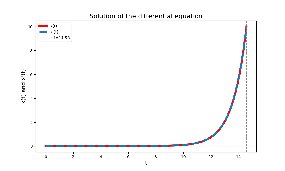
Solution obtained numerically by python Free final state with fixed final time
- Problem statement:
- Boundary conditions:
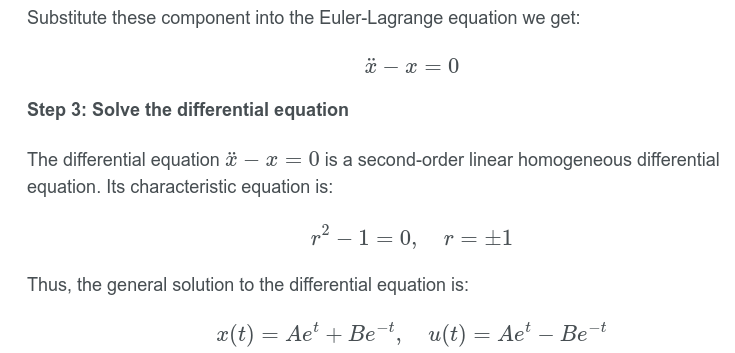
Snippet from one of the other blogs on Euler-Lagrange Equation As shown in the picture above, \(A + B = 0\), and since at \(\dot{x}(t_f)\), \(Ae^{t_f} + Be^{-t_f} = 0\), we can easily conclude that \(A = B = 0\). This means \(x(t) = 0\) at all time from \(t \in [0,1]\).
This makes sense intuitively because final state is free and \(x(0) = 0\), any \(u(t) \neq 0\) will incur a positive value on the cost function. Since there is no restriction on the \(x(1)\), the best choice is obviously staying at \(x(0) = 0\) at all time interal.
Free final state with free final time
- Problem statement:
- Boundary conditions:
For the same reason as in the previous case of free final state with fixed final time, \(x(t) = 0\) for \(t \in [0, t_f]\). This also makes sense intuitively because both final time and final state is free and \(x(0) = 0\), any \(u(t) \neq 0\) will incur a positive value on the cost function. Since there is no restriction on both \(x(t_f)\) and \(t_f\), the best choice is applying no control input and make the \(t_f\) as small as possible.
Introducing the control input and terminal cost
Now we introduce the control input \(u(t)\) and the terminal cost function \(\Phi(x(t_f), t_f)\) and Let’s derive the expression for the most general case that allow both free final state and free final time. First of all, the optimization problme is formulated as follows:
\[J[x,u] = \int_0^{t_f} L(x(t), u(t)) \, dt + \Phi(x(t_f), t_f)\] \[\text{s.t.} \quad \dot{x}(t) = f(x(t), u(t)), \quad x(0) = x_0\]To handle the equality constraints due to system dynamcis, we introduce the lagrange multiplier \(\lambda\) (which is also a function of time) and reformulate the objective functional:
\[J[x,u,\lambda] = \int_0^{t_f} \left[ L(x(t), u(t)) + \lambda^T(t) (f(x(t), u(t)) - \dot{x}(t)) \right] dt + \Phi(x(t_f), t_f)\]Define the Lagrangian \(\mathcal{L} = L(x,u) + \lambda^T (f(x,u) - \dot{x}(t))\) and the first variation is:
\[\delta J^*[x,u,\lambda] = \int_0^{t_f} \left[ \left( \nabla_x \mathcal{L}^* - \frac{d}{dt} \nabla_{\dot{x}} \mathcal{L}^* \right) \delta x + \nabla_u \mathcal{L}^* \delta u \right] dt\] \[+ \nabla_{\dot{x}} \mathcal{L}^*\big|_{t_f} \delta x_{f} + \left[\mathcal{L}^*\big|_{t_f} - \nabla_x \mathcal{L}^*\big|_{t_f}\dot{x}^*(t_f)\right] \delta t_f\] \[+ \nabla_x \Phi^* \big|_{t_f} \delta x_{f} + \frac{\partial \Phi^*\big|_{t_f}}{\partial t_f} \delta t_f\]where \(\nabla_{\dot{x}} \mathcal{L}^*\big|_{t_f} \delta x_{f}\) comes from integration by part, similiar to the previous derivation of Euler-Lagrange Equation.Rearrange the term to separate \(\delta t, \delta x_{f}, \text{and } \delta t_{f}\):
\[\delta J^*[x,u,\lambda] = \int_0^{t_f} \left[ \left( \nabla_x \mathcal{L}^* - \frac{d}{dt} \nabla_{\dot{x}} \mathcal{L}^* \right) \delta x + \nabla_u \mathcal{L}^* \delta u \right] dt\] \[+ \left[ \nabla_{\dot{x}} \mathcal{L}^*\big|_{t_f} + \nabla_x \Phi^* |_{t_f}\right]\delta x_{f}\] \[+ \left[ \mathcal{L}^*\big|_{t_f} - \nabla_x \mathcal{L}^*\big|_{t_f}\dot{x}^*(t_f) + \frac{\partial \Phi^*\big|_{t_f}}{\partial t_f}\right] \delta t_f\]Thus, when encounters an optimal control problem, the general procedures can be think of as the following:
def Brain(problem_setting):
  # Determine the type of optimal control problem
  return delta_xf, delta_tf

problem_solved = False
delta_xf, delta_tf = Brain(problem_setting)
while problem_solved is not True:
  # For fixed final state case
  if delta_xf is 0:
    # directly use the given final state value
  # For free final state case
  else:
    # solve the following equations
  # For free final time case
  if delta_tf is not 0:
    # solve the following equations
problem_solved = True # Hopefully
We now introduce the Control Hamiltonian (minimum) to make the expression more compact and the different formulation of Control Hamiltonian will be discussed in the later section of this blog:
\[\mathcal{H}(\mathbf{x}(t), \mathbf{u}(t), \mathbf{\lambda}(t)) = L(\mathbf{x}(t), \mathbf{u}(t)) + \mathbf{\lambda}^T(t)f(\mathbf{x}(t), \mathbf{u}(t))\] \[\dot{x}^* = \nabla_{\lambda}\mathcal{H}^*(x^*(t), u^*(t), \lambda^*(t))\] \[\dot{\lambda}^* = -\nabla_{x}\mathcal{H}^*(x^*(t), u^*(t), \lambda^*(t))\]Example 2: Continuous LQR and ARE
Consider the following final horizon and free final state LQR problem desribed as follows. We will show that Algebraic Riccati Equation (ARE) can be derived using the previously mentioned procedures as \(T \to \infty\).
\[J = \frac{1}{2} \int_{0}^{T} (x(t)^TQx(t) + u(t)^TRu(t)) \, dt + \frac{1}{2} x(t)^T H x(t)\] \[s.t. \quad \dot{x} = Ax(t) + Bu(t)\]where \(Q > 0\), \(R \geq 0\) and \(H\) is a constant positive definite matrix.
- Formulate Control Hamiltonian:
- Construsct state and co-state equations:
- Obtaining Optimal \( u \):
Since we are NOT concerned with the control input constraints here, the optimal control input \(u\) can be directly obtained by setting the following equation to zero.
\[\nabla_u{\mathcal{H}} = Ru + B^T\lambda = 0, \quad u^* = -R^{-1}B^T\lambda\]Substitute \(u^*\) into state equation and put them all together into matrix form:
\[\begin{bmatrix} \dot{\mathbf{x}}^*(t) \\ \dot{\mathbf{\lambda}}^*(t) \end{bmatrix} = \begin{bmatrix} A & -B R^{-1} B^T \\ -Q & -A^T \end{bmatrix} \begin{bmatrix} \mathbf{x}^*(t) \\ \mathbf{\lambda}^*(t) \end{bmatrix}\]Now suppose the costate \(\lambda\) is linearly dependent on state \(x\) (See Appendix for more detail about the validation of this assumption), and its time derivative can be expressed as follows:
\[\mathbf{\lambda}^*(t) = \mathbf{P}(t) \mathbf{x}^*(t)\] \[\dot{\mathbf{\lambda}}^*(t) =\dot{\mathbf{P}}(t) \mathbf{x}^*(t) + \mathbf{P}(t) \dot{\mathbf{x}}^*(t)\]where \(P(t)\) is a time varying matrix. Substitute into state space representation:
\[\begin{bmatrix} \dot{\mathbf{x}}^* \\ \dot{P}\mathbf{x}^* + P\dot{\mathbf{x}}^* \end{bmatrix} = \begin{bmatrix} A & -B R^{-1} B^T \\ -Q & -A^T \end{bmatrix} \begin{bmatrix} \mathbf{x}^*(t) \\ \mathbf{\lambda}^*(t) \end{bmatrix}\]- Differntial Riccati Equation (DRE) and Algebraic Riccati Equation (ARE):
From costate equation, we can obtain:
\[\dot{\lambda}^* = \dot{P}x^* + P(Ax^* - BR^{-1}B^{T}Px^*) = -Qx^* - A^{T}Px^*\] \[\dot{P}x^* + PAx^* - PBR^{-1}B^{T}Px^* = -Qx^* - A^{T}Px^*\] \[\dot{P} + PA + A^{T}P - PBR^{-1}B^{T}P + Q = 0 \tag{1} \label{eq:DRE}\]Now, we get the DRE \eqref{eq:DRE} that \(P(t)\) evolves accroding to. For a stable system, when \(T\) (upper limit of integral) approachs infinity, matrix \(P(t)\) also converges to a constant value and \(\dot{P}(t)\) becomes to zero (See Appendix for more detail about the validation of this assumption). This give rises to the ARE:
\[PA + A^{T}P - PBR^{-1}B^{T}P + Q = 0 \tag{2} \label{eq:ARE}\]- Boundary conditions:
We have \(2n\) first order differential equations (\(n\) from the \(x\) and \(n\) from \(\lambda\)), so we need \(2n\) boundary conditions to solve the problem. Given initial condition of \(x_0\), we have \(n\) boundary conditions at the initial time of state equation.
Recall we are dealing with the type of free final state fixed final time problem. Equipped with the tool we just derived from previous section, the other \(n\) boundary conditions for this type of problem can be obtained by setting the term in front of \(\delta x_f\) to zero.
\[\nabla_{\dot{x}} \mathcal{L}^*\big|_{t_f} + \nabla_x \Phi^* |_{t_f} = 0\]where
\[\mathcal{L}^* = \frac{1}{2} (x^{*T}Qx^* + u^{*T}Ru^*) + \lambda^T (Ax^* + Bu^* - \dot{x}^*)\] \[\Phi^* |_{t_f} = \frac{1}{2} (x^{*T}(t_f)Hx^*(t_f))\] \[-\lambda^*(t_f) + Hx^*(t_f) = 0 , \quad \lambda^*(t_f) = Hx^*(t_f)\]Thus, the other \(n\) boundary conditions come from the costate state equation at the final time and we need to solve the ARE backward in time to get costate trajectory \(\lambda^*(t)\). Then the optimal control input trajectory \(u^*(t)\) can obtained by the preivously derived optmality condition (\(u^*(t) = -R^{-1}B^T\lambda^*(t)\)).
Pontryagin’s Maximum Principle
- Continuous time PMP For a given system an a give optimal criterion, let \(u^* \in \mathcal{U}\) be an optimal control, then there is a variable called costate which together with the state variables satifsfies the Hamilton canonical equations. In addition, it turns out Pontryagin’s Maximum Principle is also frequently refered as Pontryagin’s Minimum Principle. The difference comes from the different formulasim of the Control Hamiltonian. For Pontryagin’s Maximum Principle, the Control Hamiltonian (maximum) is defined as follows:
\[\mathcal{H}(\mathbf{x}(t), \mathbf{u}(t), \mathbf{\lambda}(t), t) = -L(\mathbf{x}(t), \mathbf{u}(t)) + \mathbf{\lambda}^T(t)[f(\mathbf{x}(t), \mathbf{u}(t))]\] \[\dot{x}^* = \nabla_{\lambda}\mathcal{H}(x^*(t), u^*(t), \lambda^*(t), t)\] \[\dot{\lambda}^* = -\nabla_{x}\mathcal{H}(x^*(t), u^*(t), \lambda^*(t), t)\] \[u^* = \arg \max_{u \in \mathcal{U}} H(x(t)^*, u(t), \lambda(t)^*, t)\]For Pontryagin’s Minium Principle, the Control Hamiltonian (minimum) is defined as follows:
\[\mathcal{H}(\mathbf{x}(t), \mathbf{u}(t), \mathbf{\lambda}(t), t) = L(\mathbf{x}(t), \mathbf{u}(t)) + \mathbf{\lambda}^T(t)[f(\mathbf{x}(t), \mathbf{u}(t))]\]This results in the optimal control is the one that minimize the Control Hamiltonian:
\[u^* = \arg \min_{u \in \mathcal{U}} H(x(t)^*, u(t), \lambda(t)^*, t)\]- Corollaries [8]
Pontryagin and his co-workers have also derived other necessary conditions for optimality that we will find useful. We now state, without proof, two of these necessary conditions:
If the final time is fixed and the Hamiltonian does not depend explicitly on time, then the Hamiltonian must be a constant when evaluated on an extremal trajectory; that is,
\[\mathcal{H}(x^*(t), u^*(t), \lambda^*(t)) = c_1 \quad \text{for} \; t \in [t_0, t_f].\]If the final time is free, and the Hamiltonian does not explicitly depend on time, then the Hamiltonian must be identically zero when evaluated on an extremal trajectory; that is,
\[\mathcal{H}(x^*(t), u^*(t), \lambda^*(t)) = 0 \quad \text{for} \; t \in [t_0, t_f].\]
- Discrete time PMP and KKT [2]
In discrete time setting, the PMP can be viewed as a special case of Karush–Kuhn–Tucker conditions (KKT), check out the second reference for more details from Prof. Zac Manchester. Let’s first take a look at the optimization problem formulated as follows:
\[\min_{x_k, u_k} \sum_{k=0}^{N-1} L(x_k, u_k) + \Phi(x_N)\] \[s.t. \quad x_{k+1} = f(x_k, u_k)\]Same as before, \(f(x_k, u_k)\) defines the system dynamics and \( L(x_k, u_k), \Phi(x_N)\) are stage cost and terminal cost function respectively. We can then formulate the Lagrangian and proceed the procedure in the KKT manner:
\[\mathcal{L} = \sum_{k=0}^{N-1} \left[ L(x_k, u_k) + \lambda_{k+1}^\top \left( f(x_k, u_k) - x_{k+1} \right) \right] + \Phi(x_N) \tag{3} \label{eq:Lagrangian}\] \[\frac{\partial \mathcal{L}(x_k, u_k)}{\partial \lambda_{k+1}} = f(x_k, u_k) - x_{k+1} = 0 \quad (k = 0, \cdots ,N-1) \tag{4} \label{eq:state}\] \[\frac{\partial \mathcal{L}}{\partial x_k} = \frac{\partial L(x_k, u_k)}{\partial x_k} + \left( \frac{\partial f(x_k, u_k)}{\partial x_k} \right)^\top \lambda_{k+1} - \lambda_k \\(k = 1, ..., N-1 \\) \tag{5} \label{eq:costate}\] \[\frac{\partial \mathcal{L}}{\partial x_N} = \frac{\partial \Phi(x_N)}{\partial x_N} - \lambda_N \quad \\(k = N \\) \tag{6} \label{eq:boundary}\]To clarify the dimensions of each equations, suppose \(x\) has \(n\) elements, which is a (\( n \times 1 \)) vector at each time step \(k\) (and so is \(\lambda\)), and there are \( k = N\) time step. At each time step \(k \), the partial derivative of Lagrangian
- w.r.t \( \lambda_{k+1}\) is a \( n \times 1 \) column vector. From \(k = 0 \cdots N-1\), results in \(n \times N\) equations. Note that we are also given \(x_0\), which is a boundary condition at \(k = 0 \) with dimension \(n \times 1\).
- w.r.t \( x_k\) is a \( n \times 1 \) column vector. From \(k = 1, \cdots, N\), results in \(n \times (N-1)\) euqations.
Since \(x_k\) is a \(n \times 1\) column vector, \( f(x_k, u_k) \) is a also a vector, so its Jacobian matrix (\(n \times n\))with respect to \( x_k \) is given by:
\[\frac{\partial f(x_k, u_k)}{\partial x_k} = \begin{bmatrix} \frac{\partial f_1}{\partial x_{k1}} & \frac{\partial f_1}{\partial x_{k2}} & \cdots & \frac{\partial f_1}{\partial x_{kn}} \\ \frac{\partial f_2}{\partial x_{k1}} & \frac{\partial f_2}{\partial x_{k2}} & \cdots & \frac{\partial f_2}{\partial x_{kn}} \\ \vdots & \vdots & \ddots & \vdots \\ \frac{\partial f_n}{\partial x_{k1}} & \frac{\partial f_n}{\partial x_{k2}} & \cdots & \frac{\partial f_n}{\partial x_{kn}} \end{bmatrix}\]The term \(-\lambda_k\) appears because \(x_k\) is also present in term \(\lambda_k^\top \left( f(x_{k-1}, u_{k-1}) - x_{k} \right)\) from the previous time step \(k-1\), thus:
\[\begin{bmatrix} \frac{\partial \lambda_{k+1}^\top \left( f(x_k, u_k) - x_{k+1} \right)}{\partial \lambda_{(k+1)1}} \\ \frac{\partial \lambda_{k+1}^\top \left( f(x_k, u_k) - x_{k+1} \right)}{\partial \lambda_{(k+1)2}} \\ \vdots \\ \frac{\partial \lambda_{k+1}^\top \left( f(x_k, u_k) - x_{k+1} \right)}{\partial \lambda_{(k+1)n}} \end{bmatrix} = \frac{\partial \mathcal{L}(x_k, u_k)}{\partial x_k}^\top \lambda_{k+1}\]- w.r.t \( x_N\) is a \( n \times 1 \) column vector, which is a boundary condition at \(k = N \).
- We can make the above expression more compact by defining the Control Hamiltonian (in discrete time):
The Langrangian function \eqref{eq:Lagrangian} can be then rewritten as:
\[\mathcal{L} = L(x_0, u_0) + \lambda_{1}^\top f(x_k, u_k) + \sum_{k=1}^{N-1} \left[ L(x_k, u_k) + \lambda_{k+1}^\top f(x_k, u_k) - \lambda_{k}^\top x_{k+1} \right] + \Phi(x_N) - \lambda_{N}^\top x_N\] \[\mathcal{L} = H_0 (x_0, u_0, \lambda_{1}) + \sum_{k=1}^{N-1} \left[ H_k (x_k, u_k, \lambda_{k+1}) - \lambda_{k}^\top x_k \right] + \Phi(x_N) - \lambda_{N}^\top x_N\]The stationarity condition requires the gradient of the Lagrangian with respect to both (x_k) and (u_k) to be zero:
\[\nabla_{x_k, u_k} \mathcal{L} = 0\]The stationarity condition in the KKT framework involves taking the gradient of the Lagrangian with respect to the decision variables (both \(x_k\) and \(u_k\)) and setting it to zero. This ensures that the Lagrangian is stationary (i.e., no change) at the optimal solution.
In the context of PMP, the stationarity condition with respect to the control variable (u_k) is used to derive the optimality condition for the control:
- State Equation (Primal Feasibility:): (rearranging \eqref{eq:state})
- Costate Equation (Dual Feasibility & Resulting From Stationarity Condition): (rearranging \eqref{eq:costate})
Recall that we denote the initial boundary condition at \( k = 0 \) by \( x_0 \) and the terminal boundary condition at \( k = N \) by \( \lambda_N \). The boundary conditions at each intermediate point must also be satisfied. For instance, \( x_1 \) exists in two equations (\( x_1 = f(x_0, u_0) \) and \( x_2 = f(x_1, u_1) \)), and it must be consistent and satisfy both equations. Therefore, we have as many equations as boundary conditions to solve the problem. In addition, notice that \(\lambda_{k+1}^* \) is on the right and \( \lambda_{k}^*\) is on left. This indicates that the costate equation is evolving backward in time .
- Optimality Condition (Resulting From Stationarity Condition):
In the case of there is no control input constraint, we can just take the partial derivative of the Control Hamiltonian w.r.t. \(u_k\) and set is to zero:
\[\frac{\partial H_k^*}{\partial u_k^*} = 0\]In the case of control input constraint exits, we need to find the control input within the admissible set that minimize the Control Hamiltonian:
\[u_k^* = \arg \min_{u_k \in \mathcal{U}} H_k (x_k^*, u_k^*, \lambda_{k+1}^*)\]Example 3: Constrained Cotinuous LQR [1]
Consider the LQR in continuous time setting, the objective function to be minimized is defined as follows:
\[\min_{x(t), u(t)} \frac{1}{2} \int_{0}^{t_f} \left( x^T(t) Q x(t) + u^T(t) R u(t) \right) dt\] \[s.t. \quad \dot{x}(t) = A x(t) + B u(t),\] \[\quad x(0) = r_0, \quad x(t_f) = r_f, \quad u \in \mathcal{U}\]where \(Q > 0, R \geq 0\). In this case, Let’s use the Pontryagin’s Maximum Principle, so the Control Hamiltonian (maximum) is defined as:
\[H = - \frac{1}{2} x^T Q x - \frac{1}{2} u^T R u + \lambda^T (A x + B u)\]The optimal \(u^*\) in case of no control input constraint can be obtained by
\[\nabla_{u} \mathcal{H} = 0, \quad u^* = u_{LQR} = -R^{-1}B^T\lambda^*\]In the case of there exists control input consraints, based on Pontryagin’s Maximum Principle:
\[\cancelto{}{-\frac{1}{2} {x^*}^T Q x^{*}} - \frac{1}{2} {u^*}^T R u^* + \cancelto{}{\lambda^{*T} A x^{*}} + \lambda^{*T} B u^*\] \[\geq \cancelto{}{-\frac{1}{2} {x^*}^T Q x^{*}} - \frac{1}{2} u^T R u + \cancelto{}{\lambda^{*T} A x^{*}} + \lambda^{*T} B u, \quad u \in \mathcal{U}\] \[- \frac{1}{2} u^{*T} R u^* + \lambda^{*T} B u^* \geq - \frac{1}{2} u^T R u + \lambda^{*T} B u, \quad u \in \mathcal{U}\] \[u^* = \arg\max_{u \in \mathcal{U}} \left[ - \frac{1}{2} u^T R u + \lambda^{*T} B u \right]\]For scalar case (first-ordered and single-input system):
\[u^*(t) = \arg\max_{u_{\min} \leq u(t) \leq u_{\max}} \left[ - \frac{1}{2} r u(t)^2 + b \lambda^*(t) u(t) \right]\] \[u^* = \begin{cases} \frac{b \lambda^*}{r} & \text{if } u_{\min} \leq \frac{b \lambda^*}{r} \leq u_{\max} \\ u_{\min} & \text{if } \frac{b \lambda^*}{r} < u_{\min} \\ u_{\max} & \text{if } \frac{b \lambda^*}{r} > u_{\max} \end{cases}\] \[u^*(t) = \text{sat}_{u_{\min}}^{u_{\max}} \left( \frac{b \lambda^*(t)}{r} \right)\]Substitute into the Hamilton canonical equations (state and costate equations)
\[\dot{x} = a x + b \, \text{sat} \left( \frac{b \lambda^*(t)}{r} \right)\] \[\dot{\lambda} = - a \lambda + q x\]In general, the opitmal control input cannot be obtained by simply staurate the optimal unconstrained LQR output.
\[u^* \neq \text{sat}(u_{\text{LQR}})\]Summary
- One of the most important reason that make PMP crucial lies in the fact that maximizing the Hamiltonian is much easier than the original infinite-dimensional control problem. It converts the problem of maximizing over a function space to a pointwise optimization.
- ARE can be viewed be derived from the perspective of PMP, whiich is a special case when there is no constraint on control input.
- In contrast to the Hamilton–Jacobi–Bellman equation, which needs to hold over the entire state space to be valid, PMP is potentially more computationally efficient in that the conditions which it specifies only need to hold over a particular trajectory.
References
- L7.1 Pontryagin’s principle of maximum (minimum) and its application to optimal control (Explains the difference of Control Hamiltonian formulation in both Maximum and Minimum Principle)
- Optimal Control (CMU 16-745) 2023 Lecture 6: Deterministic Optimal Control Intro (Deriviation of PMP in discrete time setting, starting at 57 minutes and 15 seconds)
- Karush-Kuhn-Tucker (KKT) conditions: motivation and theorem (Part of Intro to Optimization Course by Prof. Lewis Mitchell, also contains other great explanation including lagrange multipliers, Netwon’s method, etc.)
- Hamiltonian Method of Optimization of Control Systems (Clear example problem solved using Control Hamiltonian)
- Why the Riccati Equation Is important for LQR Control (Derivation of ARE using the approach of completing the square)
- Matrix Calculus (Great explanation on matrix and vector derivatives)
- Geomety of the Pontryagin Maximum Principle (Explanation of PMP from another persepctive)
- D. E. Kirk, Optimal Control Theory: An Introduction, 2004.
Appendix
Recall from previous section, after substituing \(u^*\) and getting the boundary conditions, we obtained:
\[\begin{bmatrix} \dot{\mathbf{x}}^*(t) \\ \dot{\mathbf{\lambda}}^*(t) \end{bmatrix} = \begin{bmatrix} A & -B R^{-1} B^T \\ -Q & -A^T \end{bmatrix} \begin{bmatrix} \mathbf{x}^*(t) \\ \mathbf{\lambda}^*(t) \end{bmatrix}\] \[\lambda^*(t_f) = Hx^*(t_f)\]Based on the knowledge of the Linear System Theory, the solution can be expressed as follows:
\[\begin{bmatrix} \mathbf{x}^*(t_f) \\ \lambda^*(t_f) \end{bmatrix} = e^{A_{\text{aug}}(t_f - t)} \begin{bmatrix} \mathbf{x^*}(t_f) \\ \lambda^*(t_f) \end{bmatrix} = \begin{bmatrix} \phi_{11}(t_f - t) & \phi_{12}(t_f - t) \\ \phi_{21}(t_f - t) & \phi_{22}(t_f - t) \end{bmatrix} \begin{bmatrix} \mathbf{x^*}(t) \\ \lambda^*(t) \end{bmatrix} \\\]where
\[A_{\text{aug}} = \begin{bmatrix} A & -B R^{-1} B^T \\ -Q & -A^T \end{bmatrix}\] \[x^*(t_f) = \phi_{11}(t_f - t) x^*(t) + \phi_{12}(t_f - t) \lambda^*(t)\] \[\lambda^*(t_f) = Hx^*(t_f) = \phi_{21}(t_f - t) x^*(t) + \phi_{22}(t_f - t) \lambda^*(t)\]Substitute \(x^*(t)\) into equation of \(\lambda^*(t)\) and rearrange the equations:
\[H[\phi_{11}(t_f - t) x^*(t) + \phi_{12}(t_f - t) \lambda^*(t)] = \phi_{21}(t_f - t) x^*(t) + \phi_{22}(t_f - t) \lambda^*(t)\] \[H[\phi_{12}(t_f - t) - \phi_{22}(t_f - t)] \lambda^*(t) = [\phi_{21}(t_f - t) - H\phi_{11}(t_f - t)] x^*(t)\]Thus,
\[\lambda^*(t) = [H\phi_{12}(t_f - t) - \phi_{22}(t_f - t)]^{-1} [\phi_{21}(t_f - t) - H\phi_{11}(t_f - t)] x^*(t)\] \[\Rightarrow \mathbf{u}^*(t) = -R^{-1}B^T \mathbf{P}(t) \mathbf{x}(t)\]where,
\[\mathbf{P}(t) = \left[H\phi_{12}(t_f - t) - \phi_{22}(t_f - t)]^{-1} [\phi_{21}(t_f - t) - H\phi_{11}(t_f - t)\right]\]Given that system is stable, we can get the following:
Matrix Exponential Decay:
If \(A_{\text{aug}}\) is stable, the matrix exponential \(e^{A_{\text{aug}}(t_f - t)}\) decays exponentially as \(t_f - t\) increases. This implies that the submatrices \(\phi_{ij}(t_f - t)\) derived from \(e^{A_{\text{aug}}(t_f - t)}\) also decay exponentially.
Invertibility of the Matrix:
The stability and decay properties of the submatrices contribute to the invertibility of \(H \phi_{12}(t_f - t) - \phi_{22}(t_f - t)\). For the inverse to exist and be well-behaved, the matrix must remain nonsingular (i.e., it must not approach a singularity as \(t_f - t\) increases).
Thus, these imply that \(P(t)\) converges to a steady-state value and validate our assumption in the previous section that deriving ARE.