Implementation Details of U-Net-Segmentation-Jax
Published:
Image segmentation is a fundamental computer vision task that assigns a class label to each pixel, enabling models to separate objects from their backgrounds with pixel-level precision. This blog provides the explanation of a JAX-based U-Net implementation for pet image segmentation task using the Oxford-IIIT Pet dataset. The project starts by building a U-Net from scratch, also covering evaluation metrics such as Dice score and Intersection over Union (IoU). It also implements ResNet-based transfer learning as an U-Net encoder alternative to compare with a fully trained-from-scratch U-Net segmentation model. Corresponding repository can be found here repository.
1. Image Segmentation
Compared with image classification, which predicts one label for the whole image, and object detection, which predicts bounding boxes, segmentation provides a more detailed pixel-level understanding of object shapes and boundaries. In this project, we focus on binary semantic segmentation using U-Net. Given an input image, the model predicts a mask where each pixel is classified as either foreground or background.
1.1 Segmentation Model Categories:
Semantic Segmentation:
Semantic segmentation assigns a class label to every pixel in an image. Pixels with the same semantic meaning are grouped into the same class, but different object instances are not separated. For example, if an image contains two dogs, semantic segmentation labels both as “dog” without distinguishing between dog 1 and dog 2.
U-Net is a representative model for semantic segmentation. It uses an encoder-decoder architecture, where the encoder extracts high-level features and the decoder upsamples them back to the original image resolution. Skip connections transfer fine spatial details from the encoder to the decoder, and the basic workflow can be summarized as:
\[\text{Input Image} \rightarrow \text{Encoder} \rightarrow \text{Bottleneck} \rightarrow \text{Decoder} \rightarrow \text{Segmentation Mask}\]Instance Segmentation:
Instance segmentation extends semantic segmentation by separating different objects of the same class. Instead of only predicting that certain pixels belong to the “dog” class, it predicts a separate mask for each individual dog.
Instance segmentation models usually combine object detection and mask prediction. The model first identifies object regions, then predicts a pixel-level mask for each detected object. Mask R-CNN is a classic example. It extends Faster R-CNN by adding a mask prediction branch alongside the classification and bounding-box regression branches.
Modern YOLO models are also related to instance segmentation. Although YOLO was originally designed for fast object detection, recent versions can include a segmentation head that predicts object masks in addition to bounding boxes and class labels. The output can be summarized as:
\[\text{Input Image} \rightarrow \text{Object Boxes} + \text{Class Labels} + \text{Instance Masks}\]Panoptic Segmentation:
Panoptic segmentation combines semantic segmentation and instance segmentation into one unified task. It assigns every pixel a semantic label while also separating individual instances for countable objects.
A common distinction in panoptic segmentation is between stuff and things. “Stuff” refers to background-like regions such as sky, road, grass, or wall. These regions are usually labeled semantically but do not need separate instance IDs. “Things” refer to countable objects such as people, cars, dogs, or chairs. These objects should be separated into individual instances.
Therefore, panoptic segmentation provides a more complete scene understanding than semantic or instance segmentation alone. Its output can be summarized as:
\[\text{Input Image} \rightarrow \text{Semantic Labels for All Pixels} + \text{Instance IDs for Objects}\]Promptable / Foundation Segmentation:
Promptable segmentation models use large pretrained models to generate masks based on user-provided prompts. Instead of training a small model for one specific dataset, these models are trained on large-scale segmentation data and can generalize to many objects and scenes.
SAM, the Segment Anything Model, is a representative example. Given an image and a prompt, such as a point, bounding box, or rough mask, SAM predicts the corresponding object mask. SAM2 extends this idea to video, where a prompted object can be segmented and tracked across frames.
Compared with U-Net, SAM and SAM2 are less like task-specific models trained from scratch and more like general-purpose segmentation foundation models. The promptable segmentation workflow can be summarized as:
\[\text{Input Image} + \text{Prompt} \rightarrow \text{Segmentation Mask}\]
1.2 Metric:
For image segmentation, the model output is a predicted mask, and the ground-truth label is also a mask. Therefore, evaluation should measure how well the predicted foreground region overlaps with the true foreground region. Two commonly used metrics are Dice coefficient and Intersection over Union (IoU). Both metrics compare the overlap between the predicted mask and the ground-truth mask, but they normalize the overlap in slightly different ways.
Dice Coefficient:
The Dice coefficient measures the similarity between the predicted mask and the ground-truth mask. Let \(P\) denote the set of pixels predicted as foreground, and let \(G\) denote the set of ground-truth foreground pixels . The Dice coefficient is defined as:
\[\begin{array}{|c|} \hline \displaystyle \text{Dice}(P, G) = \frac{2|P \cap G|}{|P| + |G|} \\ \hline \end{array}\]Here, \(\lvert P \cap G \rvert\) is the number of pixels that are correctly predicted as foreground, \(\lvert P \rvert\) is the total number of predicted foreground pixels, and \(\lvert G \rvert\) is the total number of ground-truth foreground pixels . The factor of \(2\) gives more weight to the overlapping region.
In terms of true positives, false positives, and false negatives, Dice can also be written as:
\[\text{Dice} = \frac{2TP}{2TP + FP + FN}\]where \(TP\) represents correctly predicted foreground pixels, \(FP\) represents background pixels incorrectly predicted as foreground, and \(FN\) represents foreground pixels missed by the model.
The Dice score ranges from \(0\) to \(1\). A Dice score of \(1\) means perfect overlap between the predicted mask and the ground-truth mask, while a Dice score of \(0\) means no overlap. Dice is especially useful when the foreground object occupies a small portion of the image, because it directly emphasizes the overlap between predicted and true foreground regions.
IoU:
Intersection over Union, also called the Jaccard index, measures the ratio between the overlapping region and the union of the predicted and ground-truth regions. Using the same notation, where \(P\) is the predicted foreground mask and \(G\) is the ground-truth foreground mask, IoU is defined as:
\[\begin{array}{|c|} \hline \displaystyle \text{IoU}(P, G) = \frac{|P \cap G|}{|P \cup G|}\\ \hline \end{array}\]The numerator \(\lvert P \cap G \rvert\) is the intersection between the predicted mask and the ground-truth mask. The denominator \(\lvert P \cup G \rvert\) is the union of the two masks, which includes all pixels that belong to either the prediction or the ground truth.
In terms of \(TP\), \(FP\), and \(FN\), IoU can be written as:
\[\text{IoU} = \frac{TP}{TP + FP + FN}\]IoU also ranges from \(0\) to \(1\). A value of \(1\) means the predicted mask perfectly matches the ground-truth mask, while a value of \(0\) means there is no overlap. Compared with Dice, IoU is usually stricter because the union term penalizes both over-segmentation and under-segmentation more directly.
Dice and IoU are closely related. Given an IoU score, the corresponding Dice score can be computed as:
\[\text{Dice} = \frac{2 \cdot \text{IoU}}{1 + \text{IoU}}\]Similarly, given a Dice score, IoU can be computed as:
\[\text{IoU} = \frac{\text{Dice}}{2 - \text{Dice}}\]In practice, both metrics are useful for evaluating segmentation performance. Dice is often used as both an evaluation metric and a training loss, while IoU is commonly used to report the final segmentation quality.
Implementation Details (jax.vmap)
The following code snippet is used for metric calculation (
metric.py):@jax.vmap def _per_example_iou(pred_mask: jnp.ndarray, true_mask: jnp.ndarray, eps: float = 1e-6) -> jnp.ndarray: pred_mask = pred_mask.reshape(-1) true_mask = true_mask.reshape(-1) intersection = jnp.sum(pred_mask * true_mask) union = jnp.sum(pred_mask) + jnp.sum(true_mask) - intersection batch_iou = (intersection + eps) / (union + eps) return batch_iou @jax.vmap def _per_example_dice(pred_mask: jnp.ndarray, true_mask: jnp.ndarray, eps: float = 1e-6) -> jnp.ndarray: pred_mask = pred_mask.reshape(-1) true_mask = true_mask.reshape(-1) intersection = jnp.sum(pred_mask * true_mask) denom = jnp.sum(pred_mask) + jnp.sum(true_mask) return (2.0 * intersection + eps) / (denom + eps) def segmentation_metrics(logits: jnp.ndarray, labels: jnp.ndarray, threshold: float = 0.5) -> dict[str, jnp.ndarray]: # IoU/Dice need hard {0,1} preds; threshold sigmoid(logits), not raw logits. probs = jax.nn.sigmoid(logits) preds = (probs >= threshold).astype(jnp.float32) labels = labels.astype(jnp.float32) return { "iou": _per_example_iou(preds, labels).mean(), "dice": _per_example_dice(preds, labels).mean(), }For each primitive (*, sum, /, etc.), vmap defines a batched rule: “if inputs carry a batch axis, run the op so all batch elements are handled together.” Picture that describe the shape change of input argument is shown below (
pred_maskin_per_example_iou):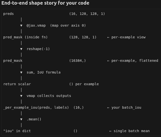
jax.vmap batch operation explanation.
2. U-Net Architecture
U-Net is a widely used encoder-decoder architecture for image segmentation. The encoder gradually downsamples the input image and extracts high-level visual features, while the decoder upsamples these features back to the original image resolution to produce a pixel-wise segmentation mask.
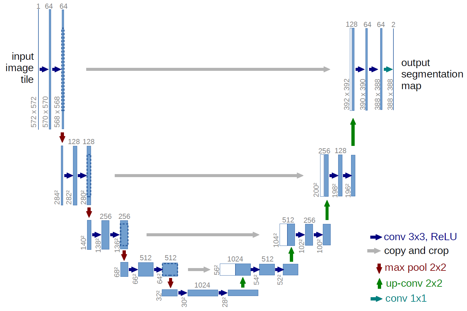
A key feature of U-Net is the skip connection between corresponding encoder and decoder stages. These connections pass low-level spatial details, such as edges and boundaries, directly to the decoder, helping the model recover fine object structures. This blog post first explains a standard U-Net architecture and then explore a transfer learning version, where a pretrained ResNet is used as the encoder. The project is written in jax, and the key function create_train_state is shown below:
def create_train_state(
    rng: jax.Array,
    config: TrainConfig,
    *,
    init_resnet_encoder_from_pretrained: bool = True,
) -> tuple[TrainState, nn.Module]:
    dummy = jnp.ones((1, config.image_size, config.image_size, 3), dtype=jnp.float32)
    if config.use_resnet:
        model: nn.Module = ResNet10UNet(out_channels=1)
        variables = model.init(rng, dummy, train=False)
        if init_resnet_encoder_from_pretrained:
            rwp = (
                Path(config.resnet_weights_path).expanduser().resolve()
                if config.resnet_weights_path
                else None
            )
            variables = load_pretrained_resnet10_encoder_into_variables(
                variables,
                weights_path=rwp,
                weights_download_url=config.resnet_weights_url,
            )
    else:
        model = create_model(config.channels)
        variables = model.init(rng, dummy, train=True)
    tx = optax.adam(config.learning_rate)
    params = _unfreeze_pytree(variables["params"])
    batch_stats = _unfreeze_pytree(variables.get("batch_stats"))
    state = TrainState.create(
        apply_fn=model.apply,
        params=params,
        batch_stats=batch_stats,
        tx=tx,
    )
    return state, model
dummy is a fake one-image input tensor (1, image_size, image_size, 3) passed to model.init() so Flax can run a forward pass once, infer all layer shapes, and allocate the model’s params (and batch_stats) before real training data is used. Thus, here is use the channels-last convention for images - (N, H, W, C), where N represent batch size, H,W are height and width, C is the channels (feature depth).
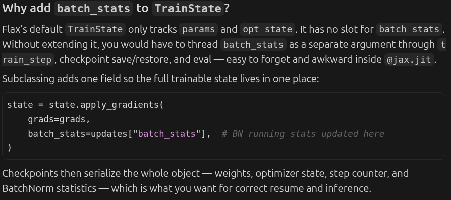
from flax.training import train_state

class TrainState(train_state.TrainState):
    batch_stats: Any
The code also uses a small extension of Flax’s built-in TrainState (flax.training.train_state), which extends it with batch_stats so BatchNorm’s running statistics are carried, updated, and checkpointed alongside the learnable parameters. In short, JAX provides arrays, transforms, and autodiff; Flax adds the neural-network layer on top, and TrainState is Flax’s standard container for everything you need during training. More details about batch_stats is shown below.
The train_step is the function that does neural network parameters update. variables is the input bundle Flax needs for a forward pass: learnable params (from the current optimization step) and batch_stats (BatchNorm running mean/variance). state.apply_fn runs the UNet on images with train=True, so BatchNorm uses batch statistics and updates its running averages. mutable=["batch_stats"] tells Flax that only batch_stats may change during this call; those changes are returned in updates, not via gradients.
@jax.jit
def train_step(state: TrainState, batch: dict[str, jnp.ndarray]) -> tuple[TrainState, dict[str, jnp.ndarray]]:
    images = batch["images"]
    # Ground-truth binary masks (collapsed trimap), not model output.
    masks = batch["masks"]

    def loss_fn(params):
        variables = {"params": params, "batch_stats": state.batch_stats}
        # Logits = pre-sigmoid scores; updates["batch_stats"] updates BatchNorm running mean/var for the next step.
        logits, updates = state.apply_fn(
            variables,
            images,
            train=True,
            mutable=["batch_stats"],
        )
        loss = total_loss(logits, masks)
        metrics = segmentation_metrics(logits, masks)
        metrics["loss"] = loss
        return loss, (updates, metrics)

    # has_aux: loss_fn returns (loss, aux); grads = ∂loss/∂params only; aux carries BN state updates and metrics.
    (loss, (updates, metrics)), grads = jax.value_and_grad(loss_fn, has_aux=True)(state.params)
    del loss
    state = state.apply_gradients(
        grads=_unfreeze_pytree(grads),
        batch_stats=_unfreeze_pytree(updates.get("batch_stats")),
    )
    return state, metrics
2.1 U-Net Encoder
For plain U-Net architecture, the
UNetclass is used and defined as follows:class UNet(nn.Module): out_channels: int = 1 channels: Sequence[int] = (32, 64, 128, 256) @nn.compact def __call__(self, x: jnp.ndarray, train: bool = True) -> jnp.ndarray: skips = [] for ch in self.channels[:-1]: x, skip = DownBlock(ch)(x, train=train) skips.append(skip) x = ConvBlock(self.channels[-1])(x, train=train) for ch, skip in zip(reversed(self.channels[:-1]), reversed(skips)): x = UpBlock(ch)(x, skip, train=train) # No sigmoid on the last conv: outputs logits; sigmoid(logits) is P(foreground) in trainer/losses/metrics. x = nn.Conv(self.out_channels, kernel_size=(1, 1), padding="SAME")(x) return xThe
ConvBlockshown below implements a standard double-convolution pattern used in U-Nets (and many segmentation models). Each “Conv → BatchNorm → ReLU” trio is one convolutional layer with normalization and nonlinearity.Running it twice back-to-back gives the network more capacity at that resolution: the first conv learns local features; the second refines them using the first layer’s output. Two 3×3 convs stacked also approximate a larger receptive field than a single 3×3, without the cost of a 5×5 kernel.
class ConvBlock(nn.Module): channels: int @nn.compact def __call__(self, x: jnp.ndarray, train: bool = True) -> jnp.ndarray: x = nn.Conv(self.channels, kernel_size=(3, 3), padding="SAME", use_bias=False)(x) x = nn.BatchNorm(use_running_average=not train)(x) x = nn.relu(x) x = nn.Conv(self.channels, kernel_size=(3, 3), padding="SAME", use_bias=False)(x) x = nn.BatchNorm(use_running_average=not train)(x) x = nn.relu(x) return x class DownBlock(nn.Module): channels: int @nn.compact def __call__(self, x: jnp.ndarray, train: bool = True) -> tuple[jnp.ndarray, jnp.ndarray]: x = ConvBlock(self.channels)(x, train=train) skip = x x = nn.max_pool(x, window_shape=(2, 2), strides=(2, 2), padding="SAME") return x, skipnn.Convarguments\(\texttt{self.channels}\) — number of output channels, or feature maps. The input channel count is inferred from \(x\).
\(\texttt{kernel_size=(3, 3)}\) — each output pixel combines information from a \(3 \times 3\) neighborhood in space.
\(\texttt{padding="SAME"}\) — pads the input so the output height and width match the input height and width when the stride is \(1\). With a \(3 \times 3\) kernel and SAME padding, the tensor shape changes as:
- \(\texttt{use_bias=False}\) — no per-channel bias is used. BatchNorm already has a learnable shift term, so the convolution bias is often omitted.
nn.max_poolarguments\(\texttt{window_shape=(2, 2)}\) — takes the maximum value over each \(2 \times 2\) patch.
\(\texttt{strides=(2, 2)}\) — moves the pooling window by \(2\) pixels each time. This creates non-overlapping patches, so the height and width are roughly halved.
\(\texttt{padding="SAME"}\) — pads the input so the output size is ceil(\(\frac{H}{2}\)), ceil(\(\frac{W}{2}\)) per dimension. For even \(H\) and \(W\), this is exactly half. For odd sizes, the output can differ by one pixel from the upsampling path, which is handled later in \(\texttt{UpBlock}\) with resizing.
Max pooling does not change the channel count. The tensor shape changes as:
\[(N, H, W, C) \rightarrow \left(N, \frac{H}{2}, \frac{W}{2}, C\right)\]
2.2 U-Net Decoder
UpBlockis the decoder counterpart toDownBlock. It upsamples the deep feature map, aligns it with a saved encoder skip, merges them, and refines with aConvBlock. In short:ConvTransposereverses the spatial halving frommax_pool; concatenation is the U-Net skip;ConvBlockmerges and compresses channels back toself.channels.class UpBlock(nn.Module): channels: int @nn.compact def __call__(self, x: jnp.ndarray, skip: jnp.ndarray, train: bool = True) -> jnp.ndarray: x = nn.ConvTranspose(self.channels, kernel_size=(2, 2), strides=(2, 2), padding="SAME")(x) if x.shape[1:3] != skip.shape[1:3]: x = jax_image_resize_like(x, skip) x = jnp.concatenate([x, skip], axis=-1) x = ConvBlock(self.channels)(x, train=train) return x def jax_image_resize_like(x: jnp.ndarray, ref: jnp.ndarray) -> jnp.ndarray: return jax_resize(x, (x.shape[0], ref.shape[1], ref.shape[2], x.shape[3])) def jax_resize(x: jnp.ndarray, shape: tuple[int, int, int, int]) -> jnp.ndarray: import jax return jax.image.resize(x, shape=shape, method="bilinear")nn.ConvTransposearguments\(\texttt{self.channels}\) — number of output feature maps, or channel depth after upsampling.
\(\texttt{kernel_size=(2, 2)}\) — learnable \(2 \times 2\) upsampling filter.
\(\texttt{strides=(2, 2)}\) — upsamples by approximately \(2 \times\) in height and width. This is the inverse of stride-\(2\) max pooling in \(\texttt{DownBlock}\).
\(\texttt{padding="SAME"}\) — padding is chosen so the spatial output is roughly \(\texttt{input_spatial} \times \texttt{stride}\) per dimension.
Transposed convolution both upsamples and learns how to reconstruct spatial detail; it is not just nearest-neighbor resizing.
3 ResNet-based Transfer Learning
This section explains how transfer learning is incorporated into the U-Net architecture. Instead of training the encoder from scratch, this method uses a pretrained ResNet as the feature extractor and keep its weights frozen during training. The ResNet encoder provides multi-level visual features learned from large-scale image data, while the U-Net decoder learns to upsample and combine these features into a pixel-wise segmentation mask.
3.1 ResNet-based U-Net Encoder
ResNet-based encoder is composed of multiple
ResNetBlock, defined as follows:class MyGroupNorm(nn.GroupNorm): """SERL ``MyGroupNorm`` (handles optional missing batch dim).""" def __call__(self, x: jnp.ndarray) -> jnp.ndarray: if x.ndim == 3: x = x[jnp.newaxis] x = super().__call__(x) return x[0] return super().__call__(x) class ResNetBlock(nn.Module): """SERL ResNet v1 block (two 3x3 convs + optional projection).""" filters: int strides: tuple[int, int] = (1, 1) dtype: Any = jnp.float32 @nn.compact def __call__(self, x: jnp.ndarray) -> jnp.ndarray: residual = x conv_kw: dict[str, Any] = { "use_bias": False, "dtype": self.dtype, "kernel_init": nn.initializers.kaiming_normal(), } y = nn.Conv(self.filters, (3, 3), self.strides, **conv_kw)(x) y = MyGroupNorm(num_groups=4, epsilon=1e-5, dtype=self.dtype)(y) y = nn.relu(y) y = nn.Conv(self.filters, (3, 3), **conv_kw)(y) y = MyGroupNorm(num_groups=4, epsilon=1e-5, dtype=self.dtype)(y) if residual.shape != y.shape: residual = nn.Conv(self.filters, (1, 1), self.strides, **conv_kw, name="conv_proj")(residual) residual = MyGroupNorm(num_groups=4, epsilon=1e-5, dtype=self.dtype, name="norm_proj")(residual) return nn.relu(residual + y)MyGroupNormsubclasses Flax Linen’snn.GroupNorm, which is a Flax layer that normalizes activations by grouping channels (not across the batch like BatchNorm).num_groupsis a standardGroupNormargument: splitCchannels intonum_groupsgroups (for instance, 4 groups × 16 channels whenC=64). Each group is normalized per spatial location.class ResNet10Encoder(nn.Module): """SERL ``ResNetEncoder`` with ``stage_sizes=(1,1,1,1)`` — multi-scale outputs (no global pool).""" stage_sizes: tuple[int, ...] = (1, 1, 1, 1) num_filters: int = 64 dtype: Any = jnp.float32 @nn.compact def __call__(self, x: jnp.ndarray) -> tuple[jnp.ndarray, jnp.ndarray, jnp.ndarray, jnp.ndarray]: ... s1 = s2 = s3 = s4 = None for i, block_size in enumerate(self.stage_sizes): for j in range(block_size): stride = (2, 2) if i > 0 and j == 0 else (1, 1) x = ResNetBlock( self.num_filters * 2**i, strides=stride, dtype=self.dtype, )(x) if i == 0 and j == block_size - 1: s1 = x # (1, 32, 32, 64) elif i == 1 and j == block_size - 1: s2 = x # (1, 16, 16, 128) elif i == 2 and j == block_size - 1: s3 = x # (1, 8, 8, 256) elif i == 3 and j == block_size - 1: s4 = x # (1, 4, 4, 512) assert s1 is not None and s2 is not None and s3 is not None and s4 is not None return s1, s2, s3, s4stage_sizesis a tuple telling you how manyResNetBlocks live in each of the four encoder stages:stage_sizesMeaning Common name (1, 1, 1, 1)1 block per stage × 4 stages = 4 blocks ResNet-10 (2, 2, 2, 2)2 blocks per stage × 4 stages = 8 blocks ResNet-18-style (3, 4, 6, 3)ResNet-34-style etc. This project fixes
(1, 1, 1, 1)to match SERL’s ResNet-10.for i, block_size in enumerate(self.stage_sizes): for j in range(block_size):i— stage index (0, 1, 2, 3)block_size—stage_sizes[i], i.e. how many blocks in that stagej— which block within the stage (0, 1, …,block_size - 1)
With
(1, 1, 1, 1), the inner loop always runs once per stage (j = 0only). The double loop is written generically so otherstage_sizeswould work without rewriting the encoder. Forstride = (2, 2) if i > 0 and j == 0 else (1, 1), this is the standard ResNet rule: downsample when entering a new stage, not on every block.3.2 ResNet-based U-Net Decoder and Trainig Weights
The ResNet decoder upsamples the deepest encoder feature s4 with transposed convolutions, merging skips s3, s2, and s1 via concatenation and ConvBlock fusion. Two extra upsampling stages (no skips) recover resolution lost in the encoder stem. A final 1×1 convolution outputs segmentation logits. Here, only the decoder is trained; encoder weights stay frozen .
One of the key function that is used for encoder weight loading is shown below:
  def _merge_encoder_params(target: dict[str, Any], source: dict[str, Any]) -> None:
    """Recursively overwrite ``target`` leaves with ``source`` where keys match."""
    for k, v in source.items():
        if k not in target:
            continue
        if isinstance(v, dict) and isinstance(target[k], dict):
            _merge_encoder_params(target[k], v)
        else:
            target[k] = jnp.asarray(np.asarray(v))
Parameters are a nested dict (pytree), not a flat list. This function walks every key in
source(the pickle). If both sides have a nested dict → recurse deeper. If both sides reach a leaf (an array) → copy pickle value intotarget. This is in-place merge intoparams_u["encoder"]— no new tree, just overwrite matching leaves.This is recursive because depth is arbitrary (module → submodule →
kernel/scale/…). Keys only in the pickle but not in the model are skipped; keys only in the model keep their random init.Loading (one-time at init)
The encoder weight is frozen during training,but there is no separate “freeze” flag when loading. Loading only copies pretrained values into the encoder slot of
params:model.init() → random weights for encoder + decoder ↓ load_pretrained_resnet10_encoder_into_variables() → overwrite params["encoder"] from pickle ↓ _unfreeze_pytree(variables["params"]) → put into TrainState (NOT “unfreeze for training”)Important:
_unfreeze_pytree/unfreeze()does not mean “start training the encoder.” It converts Flax’s immutableFrozenDictinto a plain Pythondictso Optax can update parameters. The name is about data structure mutability, not gradient freezing.Freezing (every training step)
Freezing is enforced in
train_step_frozen_encoder, selected when--use-resnet:step_fn = train_step_frozen_encoder if config.use_resnet else train_step for batch in train_bar: state, metrics = step_fn(state, batch)The actual freeze logic:
  def loss_fn(decoder_params: Any):
      params = merge_encoder_decoder_params(state.params["encoder"], decoder_params)
      ...
  (loss, (updates, metrics)), grads_decoder = jax.value_and_grad(loss_fn, has_aux=True)(state.params["decoder"])
  ...
  zero_encoder = jax.tree_util.tree_map(jnp.zeros_like, state.params["encoder"])
  full_grads = {"encoder": zero_encoder, "decoder": grads_decoder}
  state = state.apply_gradients(grads=_unfreeze_pytree(full_grads), ...)
Three mechanisms together:
value_and_gradonly onstate.params["decoder"]— autodiff never computes encoder gradients.zero_encoder— encoder gradient tree is explicitly all zeros.apply_gradients— Adam updatesparams; encoder getsparam - lr * 0→ unchanged.
So: weights are loaded in
resnet_weights.py; they are kept fixed intrainer.pylines 158–161 (and step selection at 260).
3.3 Results
Plain U-Net
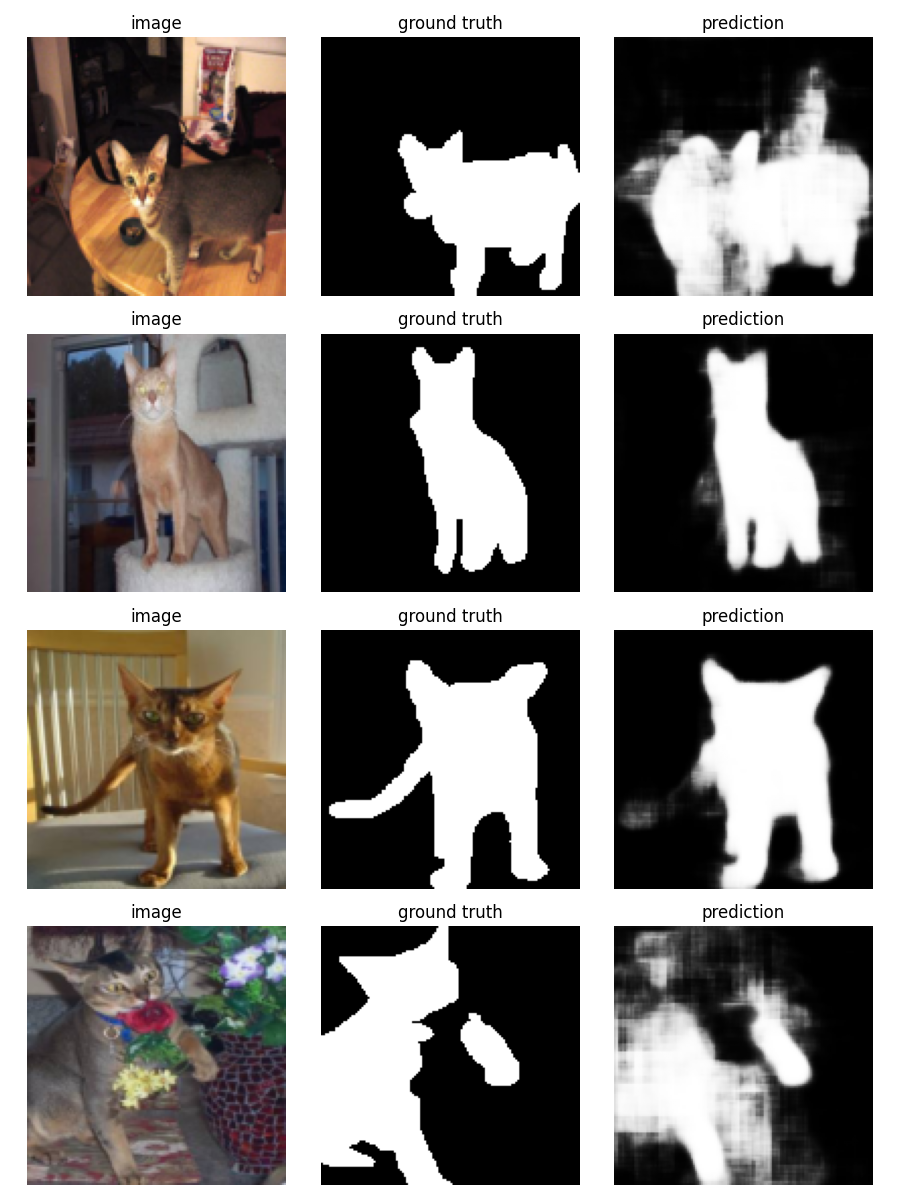
U-Net segmentation results. ResNet-based U-Net Encoder
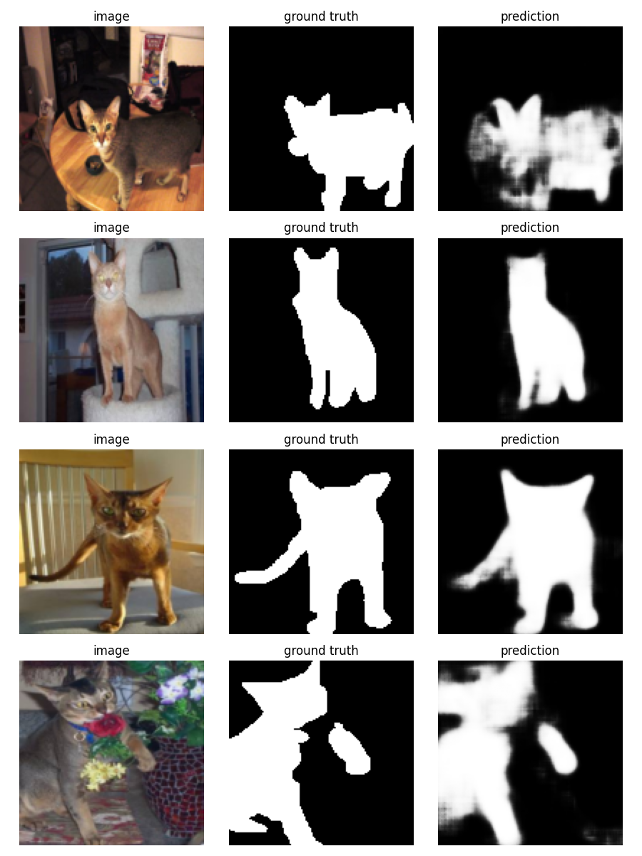
ResNet-based U-Net segmentation results.