On Derivation of Hamilton-Jacobi-Bellman Equation and Its Application

The Hamilton-Jacobi-Bellman (HJB) equation is arguably one of the most important cornerstones of optimal control theory and reinforcement learning. In this blog, we will first introduce the Hamilton-Jacobi Equation and Bellman’s Principle of Optimality. We will then delve into the derivation of the HJB equation. Finally, we will conclude with an example that shows the derivation of the famous Algebraic Riccati equation (ARE) from this perspective.

Hamilton-Jacobi Equation

In mathematics, the Hamilton–Jacobi equation is a necessary condition describing extremal geometry in generalizations of problems from the calculus of variations. It can be understood as a special case of the Hamilton–Jacobi–Bellman equation from dynamic programming.

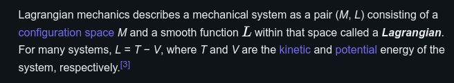
Introducing the Hamilton-Jacobi equation requires a foundational understanding of Hamiltonian mechanics and the principle of least action. Let’s begin by exploring Hamiltonian mechanics, a reformulation of classical mechanics that arises from the Lagrangian mechanics framework. The defintion of the Lagrangian \(L\) can be described as follows:

• Hamiltonian Mechanics

  • Hamiltonian (\(H\)):

    The Hamiltonian \(H\) is defined as:

    \[H(q, p, t) = p \cdot \dot{q} - L(q, \dot{q}, t)\]

    where \(L\) is the Lagrangian. \(H\) often represents the total energy of the system (kinetic + potential energy) but is formulated in terms of coordinates \(q\) and momenta \(p\).

  • Generalized Coordinates (\(q\)) and Conjugate Momenta (\(p\)):
    • \(q\) describes the configuration of the system. They can be any variables that uniquely defined the system’s state.
    • \(p\): defined as \(p = \frac{\partial L}{\partial \dot{q}}\). This is often interpreted as the momentum associated with each generalized coordinate. It is the key to the transition from Lagrangian to Hamiltonian mechanics.

  • Hamilton’s Equations of Motion:

    These are first-order differential equations that describe the time evolution of the \(q\) and \(p\):

    \[\dot{q} = \frac{\partial H}{\partial p}\] \[\dot{p} = -\frac{\partial H}{\partial q}\]

  • Phase Space and Canonical Transformations:

    • Phase space is a multidimensional space in which all possible states of a system are represented, with each state corresponding to one unique point in the phase space. For a system with n degrees of freedom, the phase space has 2n dimensions (each degree of freedom contributes one coordinate and one momentum).

    • Canonical Transformations are transformations in phase space that preserve the form of Hamilton’s equations. They are akin to coordinate transformations in classical mechanics but apply to both coordinates and momenta. Canonical transformations allow for simplifying problems or switching to more convenient variables without changing the physical content of the equations.

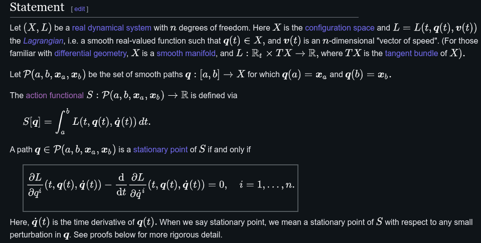
• Principle of Least Action (Hamilton’s Principle)

  • Action

    More formally, action is a mathematical functional which takes the trajectory (also called path or history) of the system as its argument and has a real number as its result. Generally, the action takes different values for different paths. Action has dimensions of energy × time or momentum × length, and its SI unit is joule-second (like the Planck constant h).

    In short, action functional returns a scalar quantity descirbes how the balance of the kinetic versus potential energy of a physical system changes with trajectory.

    \[S[q] = \int_{t_1}^{t_2} L(q, \dot{q}, t) \, dt\]

    where:

    • \(q(t)\) are the generalized coordinates.
    • \(\dot{q}(t)\) are the time derivatives of \(q(t)\) (velocities).
    • \(L(q, \dot{q}, t)\) is the Lagrangian, typically the difference between kinetic and potential energy.

  • Hamilton’s Principle and Euler-Lagrange Equation

    Hamilton’s Principle, also known as the principle of least action, states that the true path taken by a physical system between two points in time is the one that is a stationary point (a point where the variation is zero) of the action functional \(S[q]\) (note that \(q\) is a function of time).

    This means that according to Hamilton’s Principle, the actual path taken by the system makes the \(S[q(t)]\) stationary (usually a minimum). In terms of functional analysis, this implies the true evolution a phsical system is the solution of the following functional equation:

    \[\begin{array}{|c|} \hline \textbf{Hamilton's principle} \\ \frac{\delta S}{\delta q(t)} = 0. \\ \hline \end{array}\]

    This basically says that the first varition of the functional \(S\) is zero, which naturally relates to the Euler-Lagrange equations that I haved mentioned in one of the other blogs post:

    

  • Genrating Function S(q,t)

    The generating function (sometimes called Hamilton’s Principal function) \(S(q, t)\) is used in canonical transformations to change the coordinates in a way that preserves the form of Hamilton’s equations. The purpose of using \(S(q,t)\) is to simplify the Hamiltonian or to transform the problem into a more tractable form. It effectively changes both the coordinates \(q\) and \(p\).

    \(S(q, t)\) is expressed as an integral of the Lagrangian, but it represents the action evaluated along the optimal path, from the initial time \(t_1\) to time \(t_2\).

    \[S(q, t) = \int_{t_1}^{t_2} L(q(\tau), \dot{q}(\tau), \tau) \, d\tau\]

    • \(S(q, t)\) is a function of \(q\) and \(t\), because it gives a scalar value for specific values of \(q\) and \(t\).

    • The action functional \(S[q(t)]\) is different. It is a functional because it assigns a real number (the action) to a function \(q(t)\), i.e., the entire trajectory.

    Thus, the generating function \(S(q, t)\) corresponds to the trajectory \(q(t)\) for which the first variation \(\delta S[q]\) of the action functional is zero, meaning that the action is stationary (usually minimized). The Hamilton-Jacobi equation is a way to express this optimal path directly in terms of the generating function \(S(q, t)\).

• Derivation of HJ Equation

  

  After introducing the concept of Hamiltonian mechanics and principle of least action, Let’s now elaborate on the steps to derive the Hamilton-Jacobi equation:

  • Action and Hamilton’s Principal (Generating) Function:

    • The action functional \(S [q]\) is given by:
    \[S [q] = \int_{t_1}^{t} L(q, \dot{q}, t) \, d\tau\]
    • The generating function \(S(q, t)\) should make the action functional \(S[q]\) stationary (first variation is equal to zero).

  • Hamiltonian Formulation:

    • From the Lagrangian \(L\), the Hamiltonian \(H\) is defined as:

      \[H(q, p, t) = p \cdot \dot{q} - L(q, \dot{q}, t)\]

    • Here, \(p = \frac{\partial L}{\partial \dot{q}}\) are the canonical momenta.

  • Canonical Transformation:

    • Hamilton’s principal function \(S(q, t)\) serves as a generating function. This transforms the original coordinates \((q, p)\) to new ones where the Hamiltonian may take a simplified form.
  • Hamilton’s Equations:
    • The equations of motion are: \(\dot{q} = \frac{\partial H}{\partial p}\) \(\dot{p} = -\frac{\partial H}{\partial q}\)

  • Hamilton’s Principle:

    • The total differential of \(S(q,t)\) is:

      \[dS = \frac{\partial S}{\partial q} dq + \frac{\partial S}{\partial t} dt = 0\] \[\frac{dS}{dt} = \frac{\partial S}{\partial q} \dot{q} + \frac{\partial S}{\partial t} = 0\]

    • Recognizing that \(\frac{dS}{dt} = L\) thus,

      \[-\frac{\partial S}{\partial t} = \frac{\partial S}{\partial q} \dot{q} - L\] \[-\frac{\partial S}{\partial t} = H \left( q, \frac{\partial S}{\partial q}, t \right)\]

      which give rise to the Hamilton-Jacobi Equation.

      The relationship:

      \[p = \frac{\partial S}{\partial q}\]

      indicates that the new momenta \(p\) are derived from the gradient of the action with respect to the new coordinates \(q\).

Bellman’s Principle of Optimality

• Discrete time (Bellman Equation)

  Bellman equation, discrete-time counterpart of the Hamilton–Jacobi–Bellman equation.

  Bellman’s principle of optimality states that an optimal policy has the property that, regardless of the initial state and decision, the remaining decisions must form an optimal policy concerning the state resulting from the first decision.

  \[V(x_t) = \min_{u_t} \{ g(x_t, u_t) + \beta V(x_{t+1}) \}\]

  where:

  • \(V(x_t)\) is the value function representing the minimum cost-to-go from state \(x_t\).
  • \(g(x_t, u_t)\) is the immediate cost incurred at time \(t\).
  • \(\beta\) is the discount factor.
  • \(x_{t+1}\) is the state at the next time step resulting from applying control \(u_t\) to state \(x_t\).

• Continuous time (Derivation of HJB equation)

  Given the initial time \(t_0\), the optimization problem is formulated as follows:

  \[J(\mathbf{x}(t), \mathbf{u}(t), t_f) = \int_{t_0}^{t_f} \mathcal{L}(\mathbf{x}(\tau), \mathbf{u}(\tau)) d\tau + Q(\mathbf{x}(t_f), t_f)\] \[s.t. \quad \frac{d}{dt} \mathbf{x} = \mathbf{f}(\mathbf{x}(t), \mathbf{u}(t), t) \quad t \in [t_0, t_f]\]

  First, define the minimum cost-to-go function (also called as Bellman value function), since it is under the condition of optimal control \(u^*\), both state \(x(t)\) and control input \(u(t)\) trajectories are determined. Thus, it is only a function of initial state \(x_0\) and final time \(t_f\).

  \[V(\mathbf{x_0}, t_f) = \min_{\mathbf{u}(t)} J(\mathbf{x}(t), \mathbf{u}(t), t_f)\]

  Then takes its totoal derivatives:

  \[\frac{d}{dt} V(\mathbf{x_0}, t_f) = \frac{\partial V}{\partial t} + \left( \frac{\partial V}{\partial \mathbf{x}} \right)^T \frac{d \mathbf{x}}{dt}\] \[\text{L.H.S} = \min_{\mathbf{u}(t)} \frac{d}{dt} \left( \int_{0}^{t_f} \mathcal{L}(\mathbf{x}(\tau), \mathbf{u}(\tau)) d\tau + Q(\mathbf{x}(t_f), t_f) \right)\] \[= \min_{\mathbf{u}(t)} \frac{d}{dt} \left( \int_{0}^{t_f} \mathcal{L}(\mathbf{x}(\tau), \mathbf{u}(\tau)) d\tau \right)\] \[= \min_{\mathbf{u}(t)} \left(- \mathcal{L}(\mathbf{x}(\tau), \mathbf{u}(\tau)) \right)\]

  Substitute the expression of \(\frac{d \mathbf{x}}{dt}\) and since the evolution of \(x(T)\) is depend on \(u(t)\), we can incorporate it into the minimization operation that appears in the L.H.S. After rearranging the equation we get:

  \[-\frac{\partial V}{\partial t} = \min_{\mathbf{u}(t)} \left( \left( \frac{\partial V}{\partial \mathbf{x}} \right)^T \mathbf{f}(\mathbf{x}, \mathbf{u}) + \mathcal{L}(\mathbf{x}, \mathbf{u}) \right)\]

Example 1: Derivation of ARE using HJB equation

Here we derive the Algebraic Riccati Equation (ARE) from the perspective of HJB equation, check out the derivation of ARE from the perspective of Pontryagin’s Maximum Principle in this blog post with more detailed explanation. Consider the problem that is to minimize the following infinite-horizon quadratic cost function:

where:

\(Q\) is a positive semi-definite matrix (penalizes the state). \(R\), is a positive definite matrix (penalizes the control input).

where:

• \(x(t) \in \mathbb{R}^n\), is the state vector.
• \(u(t) \in \mathbb{R}^m\) is the control input.
• \(A\) and \(B\) are constant matrices of appropriate dimensions.

with the assumptions that:

• The control input is unconstrained.
• The system is controllable.

Step 1: Set Up Hamilton-Jacobi-Bellman (HJB) Equation

The HJB equation for the optimal control problem is:

Since this is an infinite-horizon problem and there is no terminal cost, with the assumption that system is controllable, the minimum cost-to-go function \(V(x,t)\) at \(t_{\infty}\) should converge. Thus, \(\frac{\partial V(x,t_{\infty})}{\partial t} = 0\), so the HJB equation simplifies to:

Step 2: Value Function Expression Assumption

Assume the value function \(V(x_0,t_{\infty})\) is quadratic in the state \(x\):

where \(P\) is a symmetric positive semi-definite matrix to be determined. Thus,

So the HJB equation becomes:

Step 3: Find Optimal Control Input \(u^*\)

To find the optimal control \(u^*\), differentiate the expression inside the minimization with respect to \(u\) and set the derivative to zero (Note that \(u\) is unconstrained):

This gives:

Solving for \(u\):

Step 4: Substitute \(u^*\) Back into the HJB Equation

Substitute \(u^* = -R^{-1} B^T P x\) into the HJB equation:

Recall P is symmetric, thus \(2PA = P A + A^T P\). Then, we can rewrite the equation as:

Step 5: Algebraic Riccati Equation (ARE)

Since this equation must hold for all \(x\), the expression inside the parentheses must be zero:

In this way, we now get the ARE.

Summary

• Function vs. Functional: While the action \(S[q(t)]\) is a functional that depends on the entire trajectory, \(S(q, t)\) is a function representing the minimized action at a specific point and time.
• Hamilton-Jacobi equation can be viewed as a special case (without control input) of Hamilton-Jacobi-Bellman (HJB) Equation. In discrete time settings, the analogous difference equation of HJB Equation is usually refered to as the Bellman Equation.
• HJB provides a fundation for both value iteration and policy iteration in continuous action spaces in the filed of reinforcement learning. Using the neural network to approximate the Bellman value function is the key of Approximate Dyanmic Programming.

References

• Nonlinear Control: Hamilton Jacobi Bellman (HJB) and Dynamic Programming (Part of excellent series on optimal control and reinforcement learning by Prof. Steve Brunton.)
• EE 564: Lecture 26 (Optimal Control): The Hamilton Jacobi Bellman Approach (Great lecture that include the derivation of ARE using HJB and connection with PMP.)
• Explaining the Principle of Least Action: Physics Mini Lesson (Include derivation of Newton’s Second Law.)
• The principle of least action
• Hamiltonian Mechanics in 10 Minutes and Understanding Hamiltonian mechanics: (1) The math (More in-depth explanation of Hamiltonian mechanics.)
• Action principle: geometric and physical interpretation