From Bigram to Transformer

Character-level name generation is a simple but effective task for understanding modern generative sequence models. This blog explains a PyTorch-based implementation that progressively builds name generators from a count-based Bigram model to Neural Bigram, MLP, RNN, GRU, LSTM, and a tiny decoder-only Transformer. Inspired by Karpathy’s makemore, the project uses a names dataset where each model learns autoregressive next-character prediction with a special start/end token. This blog post explains concepts includes embeddings, hidden states, gated memory, and causal self-attention. Implementation can be found at repository.

0. Cross Entropy Loss and Negative Log Likelihood

In this project, we want to generate names character by character. A name such as “emma” can be treated as a sequence of characters:

During training, the model does not generate the whole name at once. Instead, it learns a simpler task: given the current context, predict the next character.

For example, if the current context is:

then the model should assign a high probability to the next character:

So the core learning problem is a next-character prediction problem.

At each step, the model outputs a probability distribution over all possible characters in the vocabulary. The vocabulary may include lowercase letters and a special end token:

where “.” can represent the end of a name.

Suppose the model predicts a probability distribution \(q\) over all possible next characters, and the true next character is \(y\). The negative log-likelihood loss is:

Here, \(q(y)\) is the probability that the model assigns to the correct next character.

If the model assigns high probability to the correct character, the loss is small:

If the model assigns low probability to the correct character, the loss becomes large:

This matches our intuition: the model is punished when it is confident about the wrong prediction, and rewarded when it gives high probability to the correct next character.

Cross entropy describes a closely related idea. It measures how well a predicted distribution \(q\) matches a target distribution \(p\):

In a classification problem, the true label is usually represented as a one-hot distribution. This means the correct class has probability 1, and every other class has probability 0:

Substituting this one-hot target distribution into the cross entropy formula gives:

Therefore, for a single next-character prediction, cross entropy loss and negative log-likelihood are the same numerical quantity.

The difference is mainly about interpretation.

Negative log-likelihood comes from probability and maximum likelihood estimation. It says: we want to maximize the probability of the observed training data . Since optimization usually minimizes a loss, maximizing likelihood becomes minimizing negative log-likelihood :

Cross entropy comes from information theory and classification. It says: we want the predicted distribution \(q\) to be close to the true distribution \(p\).

So in simple terms:

Negative log-likelihood focuses on the probability assigned to the observed correct label. Cross entropy focuses on matching the predicted distribution to the target distribution. When the target is one-hot, these two views lead to the same loss.

In this name generation project, the loss is computed over many next-character predictions. For a name sequence

the training objective can be written as:

This means the model is trained to assign high probability to every correct next character in the training names.

For a bigram model, the context only contains the previous character:

For example, after seeing the character “m”, the model learns which characters are likely to come next. If names in the dataset often contain “ma”, then the model should learn a relatively high probability for:

For a neural network model, the idea is the same, but the probability distribution is produced by learnable parameters. The model first outputs logits:

where \(V\) is the vocabulary size. These logits are raw scores, not probabilities. They are converted into probabilities using softmax:

Then cross entropy compares this predicted distribution with the true next character.

In practice, libraries such as PyTorch combine softmax and negative log-likelihood into one function called cross entropy loss. This is why we usually pass raw logits directly into the cross entropy function, instead of manually applying softmax first.

This loss is important because it directly shapes the model’s generation behavior. During generation, the model starts from a special start token, predicts a distribution over the next character, samples one character, and repeats this process until it samples the end token.

Therefore, cross entropy loss is not just a training formula. It teaches the model which characters are likely to follow which contexts, and this learned probability distribution is exactly what the model uses to generate new names.

1. Bigram

The first step of this project is to build a bigram-based name generator. A bigram model is one of the simplest language models: it predicts the next character using only the current character. In other words, the model does not look at the full previous context of a name. It only learns transition probabilities such as how likely \(\text{a}\) is to appear after \(\text{m}\), or how likely the end token is to appear after \(\text{n}\).

For a character sequence

the bigram assumption writes the probability of the sequence as

This is a very strong simplification, because real names often depend on longer character patterns. For example, after seeing \(\text{ch}\), the next character distribution may be different from only seeing \(\text{h}\). However, the bigram model is still useful because it introduces the core idea of language modeling: learning a probability distribution over the next token.

In this project, two versions of the bigram model are implemented. The first version, bigram_count, directly counts how often each character follows another character in the dataset. The second version, bigram_nn, uses a small neural network to learn the same kind of next-character distribution through gradient descent. These two methods make the same modeling assumption, but they estimate the probabilities in different ways.

• 1.1 Bigram Count

  The bigram_count method builds a two-dimensional count table. Each row represents the current character, and each column represents the next character. If the vocabulary size is \(V\), then the bigram count table has shape

  \[V \times V\]

  For example, the entry at row \(\text{m}\) and column \(\text{a}\) stores how many times the transition

  \[\text{m} \rightarrow \text{a}\]

  appears in the training names. If many names contain this transition, then this count will be large. If the transition rarely or never appears, then the count will be small or zero.

  After collecting all bigram counts from the dataset, the count table can be converted into a probability table by normalizing each row:

  \[P(j \mid i) = \frac{N_{ij}} {\sum_{k=1}^{V} N_{ik}}\]

  Here, \(N_{ij}\) is the number of times character \(j\) appears after character \(i\). The denominator sums over all possible next characters after \(i\). Therefore, each row becomes a probability distribution over the next character.

  This probability table is the actual bigram language model. During generation, the model starts from a special start token, looks up the corresponding row in the probability table, samples the next character, and repeats the same process until it samples the end token.

  The main advantage of bigram_count is that it is simple and interpretable. We can directly inspect the count table and understand what the model has learned. For instance, if the row for \(\text{a}\) gives high probability to \(\text{n}\), \(\text{l}\), or the end token, then the model has learned that these are common characters after \(\text{a}\) in the training set.

  However, this method also has clear limitations. It cannot generalize beyond the observed counts. If a transition never appears in the dataset, its probability may become zero, even if the transition is still linguistically possible. Also, the model only uses one previous character as context, so it cannot capture longer patterns such as \(\text{anna}\), \(\text{ella}\), or \(\text{mar}\).

  • Note: How the NLL is calculated in bigram_count

    probs is a vocab_size × vocab_size matrix where probs[i, j] = P(next=j | current=i).

    def train_count_bigram(args: argparse.Namespace) -> None:
      train_names, val_names, _test_names, vocab = load_dataset(args.data, args.seed)
      probs = fit_bigram_counts(train_names, vocab, smoothing=args.smoothing)
      checkpoint = {
          "probs": probs,
          "vocab": vocab.to_dict(),
          "config": {"model": "bigram_count", "smoothing": args.smoothing},
      }
      Path(args.out).parent.mkdir(parents=True, exist_ok=True)
      torch.save(checkpoint, args.out)
    
      # val_x: current char ids, val_y: true next char ids (one pair per transition)
      val_x, val_y = make_bigram_examples(val_names, vocab)
      # log(probs[val_x, val_y]) returns a tensor of size [len(val_x)]
      # NLL = mean(-log P(next | current)) over validation pairs
      nll = -torch.log(probs[val_x, val_y]).mean().item()
      print(f"saved {args.out}")
      print(f"validation negative log likelihood: {nll:.4f}")
    

    This indexes one probability per validation pair: for each i, it picks P(true next | current) from the fitted table.

    Then:

    \[\text{NLL} = -\frac{1}{N}\sum_{i=1}^{N} \log P(\text{val_y}_i \mid \text{val_x}_i)\]

    In code: -torch.log(probs[val_x, val_y]).mean().

    • High probability for the true next char → small -log(p) → good
    • Low probability → large -log(p) → bad

    This is the same objective cross-entropy optimizes for bigram_nn, but here the probabilities come directly from counts rather than learned logits.

• 1.2 Bigram Neural Network

  The bigram_nn method keeps the same bigram assumption, but replaces manual counting with a learnable neural network. Instead of directly computing transition probabilities from a count table, the model learns parameters that produce logits for the next character.

  Given the current character \(x_t\), the neural network outputs a vector of logits:

  \[z = f_\theta(x_t)\]

  where \(z\) has length \(V\), the vocabulary size. Each element of \(z\) is a raw score for one possible next character. These logits are converted into probabilities using softmax:

  \[P(x_{t+1}=j \mid x_t) = \frac{\exp(z_j)} {\sum_{k=1}^{V} \exp(z_k)}\]

  The model is trained using cross entropy loss. For each training pair, the input is the current character, and the label is the next character. If the true next character is \(y\), the loss is

  \[L = -\log P(y \mid x_t)\]

  This means the model is updated to assign higher probability to the correct next character.

  In the simplest implementation, bigram_nn can be built using an embedding layer. If the vocabulary size is \(V\), an embedding layer with output dimension \(V\) can be written as

  \[\text{Embedding}(V, V)\]

  import torch
  from torch import nn
  
  class BigramNN(nn.Module):
      """A neural bigram: current character ID directly selects next-token logits."""
  
      def __init__(self, vocab_size: int):
          super().__init__()
          self.table = nn.Embedding(vocab_size, vocab_size)
  
      def forward(self, idx: torch.Tensor) -> torch.Tensor:
          # idx: [batch]
          # logits: [batch, vocab_size]
          return self.table(idx)
  

  This layer maps each input character index to a vector of length \(V\). In this project, that vector can be interpreted as the logits for the next-character distribution. Therefore, the embedding matrix plays a role similar to the bigram table, except that its values are learned by gradient descent instead of being computed by counting.

  Conceptually, bigram_count and bigram_nn are closely related. Both models learn a distribution of the form

  \[P(x_{t+1} \mid x_t)\]

  The difference is how this distribution is obtained. bigram_count estimates the distribution directly from frequency counts. bigram_nn starts from randomly initialized parameters and learns the distribution by minimizing cross entropy loss.

  This neural network version is important because it creates a bridge from simple counting-based language models to modern neural language models. Although bigram_nn is still limited to one-character context, it introduces the training pattern used later in larger models: represent tokens as indices, produce logits, apply cross entropy loss, and update parameters with backpropagation. This same basic workflow will later extend naturally to MLPs, RNNs, LSTMs, and Transformers.

2. Recurrent Neural Network (RNN)

The key idea of an RNN is that the model processes a sequence one step at a time. At time step \(t\), the model receives the current input character \(x_t\) and the previous hidden state \(h_{t-1}\). It then produces a new hidden state \(h_t\):

Here, \(x_t\) represents the current character input, \(h_{t-1}\) stores information from previous characters, and \(h_t\) becomes the updated memory after reading the current character. The function \(g\) is usually a nonlinear activation function such as \(\tanh\).

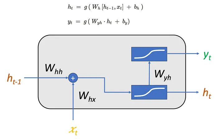
The first figure shows this recurrent computation inside a single RNN cell. The important part is that the hidden state has a loop-like structure: the previous hidden state \(h_{t-1}\) is fed into the current step, and the current hidden state \(h_t\) will be passed to the next step. This is what allows the model to carry information across the sequence.

After computing \(h_t\), the model uses it to predict the next character. In a name generation task, the output should be a distribution over all possible characters in the vocabulary. Therefore, we first compute logits:

Then we convert the logits into probabilities using softmax:

where \(V\) is the vocabulary size. This probability distribution tells us which character is likely to appear next after the current prefix.

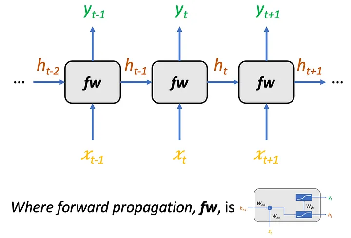
The second figure shows the same RNN cell unrolled across time. Instead of thinking of the RNN as a loop, we can expand it into a chain of repeated computations:

Each small block in the figure represents the same recurrent function. The parameters are shared across all time steps, which means the model uses the same rule to update its hidden state no matter where it is in the name.

In this project, the RNN is trained as a next-character prediction model. Given a training name such as \(\text{emma}\), we can create input-target pairs by shifting the sequence:

The start token tells the model to begin generating a name, and the end token tells the model when the name is complete. At each time step, the model predicts the target character from the current input character and the hidden state.

The training loss is still cross entropy loss. For each time step, if the correct next character is \(x_{t+1}\), the loss is

For the whole sequence, we average the loss across all time steps:

Compared with the bigram model, the main difference is the context. The bigram model predicts

while the RNN predicts

In practice, the RNN does not store the full sequence explicitly. Instead, it compresses the previous characters into the hidden state \(h_t\). This hidden state acts like a learned memory of the prefix.

During generation, the process is similar to the bigram model but with an additional hidden state. The model starts with the start token and an initial hidden state, usually initialized to zeros. It predicts a probability distribution over the next character, samples one character, updates the hidden state, and repeats this process until it samples the end token.

3. Gated Recurrent Unite (GRU)

In vanilla RNN, the hidden state is repeatedly updated through time, information from earlier characters may gradually fade away. This is especially related to the vanishing gradient problem: during backpropagation through many time steps, gradients can become very small, making it difficult for the model to learn long-range dependencies.

In the opposite case, gradients may also become too large, leading to the exploding gradient problem. Exploding gradients can often be controlled with gradient clipping, but vanishing gradients are harder because they directly affect the model’s ability to remember earlier context.

A simple RNN updates its hidden state at every step using one direct transformation, so it has limited control over what information should be preserved and what information should be overwritten.

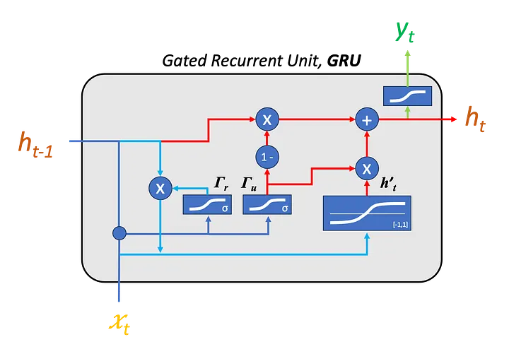
GRU improves the vanilla RNN by adding gates to control the hidden state update. The attached figure shows that a GRU cell is not just a direct update from \(h_{t-1}\) to \(h_t\). Instead, it computes several intermediate quantities that decide how much past information to keep and how much new information to write into memory.

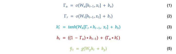
At time step \(t\), the GRU receives the current input \(x_t\) and the previous hidden state \(h_{t-1}\). It first computes a reset gate:

The reset gate controls how much of the previous hidden state should be used when forming the candidate hidden state. If part of \(\Gamma_r\) is close to \(0\), the model suppresses the corresponding part of the old memory. If it is close to \(1\), the model keeps that information.

Then the GRU computes a candidate hidden state:

Here, \(\odot\) denotes element-wise multiplication. This equation means that the model first filters the previous hidden state using the reset gate, and then combines the filtered memory with the current input to produce a candidate update.

The second important gate is the update gate:

The update gate decides how much of the old hidden state should be kept and how much should be replaced by the candidate hidden state. The final hidden state is computed as:

This equation is the core of the GRU. The new hidden state \(h_t\) is a learned mixture of the previous hidden state \(h_{t-1}\) and the candidate hidden state \(h'_t\). If \(\Gamma_u\) is close to \(0\), the model mostly keeps the old memory. If \(\Gamma_u\) is close to \(1\), the model mostly writes new information.

Compared with a vanilla RNN, this gated update gives the model a more flexible memory mechanism. Instead of always overwriting the hidden state, the GRU can preserve useful information across multiple time steps. This helps reduce the difficulty of learning longer dependencies and makes the model more stable than a simple RNN.

The main difference is that the GRU has better control over memory. The reset gate helps decide which previous information is relevant for the current step, while the update gate controls how much memory should be carried forward. As a result, the GRU can usually learn more stable character patterns than a vanilla RNN and generate names that are more coherent.

4. Long-Short Term Memotry (LSTM)

LSTM, is another recurrent architecture designed to improve the memory limitations of vanilla RNNs. Like GRU, it uses gates to control information flow, but it introduces a more explicit memory variable called the cell state, denoted as \(c_t\). Instead of storing all sequence information only in the hidden state \(h_t\), the LSTM maintains a separate memory path that can carry information across many time steps.

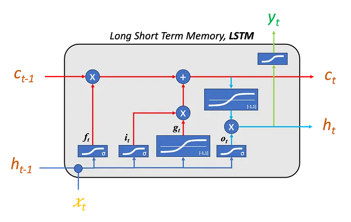
The attached figure shows two types of states inside the LSTM cell. The hidden state \(h_t\) is used for prediction and passed to the next step, while the cell state \(c_t\) acts as a longer-term memory. The horizontal path from \(c_{t-1}\) to \(c_t\) represents this memory flow. The gates decide what information should be forgotten, what new information should be written, and what part of the memory should be exposed as the hidden state.

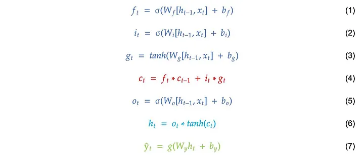
At time step \(t\), the LSTM receives the current input \(x_t\) and the previous hidden state \(h_{t-1}\). It first computes the forget gate:

The forget gate decides how much of the previous cell state \(c_{t-1}\) should be kept. If a component of \(f_t\) is close to \(0\), that part of the old memory is mostly removed. If it is close to \(1\), that information is preserved.

Next, the LSTM computes the input gate and the candidate memory:

The candidate memory \(g_t\) contains new information that could be added to the cell state, while the input gate \(i_t\) controls how much of this new information should actually be written.

The cell state is then updated as:

This equation summarizes the main idea of LSTM memory. The new cell state combines preserved old memory and selected new memory. Compared with a vanilla RNN, this additive memory update makes it easier for information and gradients to flow across time, which helps reduce the vanishing gradient problem.

Finally, the LSTM computes the output gate:

The hidden state is produced from the cell state:

This means the cell state stores the internal memory, while the output gate controls how much of that memory becomes visible through the hidden state.

Compared with GRU, LSTM has a slightly more complex structure because it separates the cell state \(c_t\) and hidden state \(h_t\). The forget, input, and output gates give the model fine-grained control over memory. For name generation, this helps the model keep useful prefix information while updating its internal representation as new characters are generated.

5. Transformer

RNN, GRU, and LSTM process a name sequentially. At each time step, the model reads one character, updates its hidden state, and then moves to the next character. This design is natural for sequence modeling, but it also has a limitation: the computation at time step \(t\) depends on the result from time step \(t-1\). Therefore, the model cannot process all positions in parallel during training in the same way that a Transformer can.

This sequential structure is one reason recurrent models are harder to scale. Even though GRU and LSTM improve the memory mechanism with gates, they still pass information through a chain of hidden states. Long-range information must travel step by step through the sequence, which can make optimization difficult. GRU and LSTM reduce the vanishing gradient problem, but they do not completely remove the sequential bottleneck.

The Transformer takes a different approach. Instead of updating a hidden state from left to right, it uses attention to let each token directly look at other tokens in the context. In name generation, this means that when predicting the next character, the model can compare the current position with previous characters in the prefix and decide which positions are most relevant.

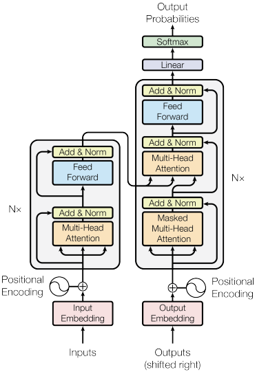
The first attached figure shows the original Transformer architecture, which contains both an encoder and a decoder. The encoder processes the input sequence, while the decoder generates the output sequence. However, for this name generation project, we do not need the full encoder-decoder structure. We only need an autoregressive model that predicts the next character from previous characters. Therefore, the implementation is a decoder-only Transformer.

This is similar in spirit to GPT-style language modeling. The model receives a prefix such as

and predicts the next character distribution based only on the characters that have already appeared. It should not be allowed to look at future characters during training. This is why the model uses causal self-attention.

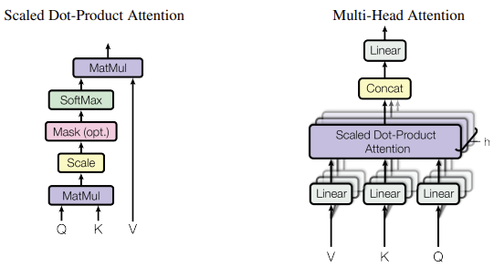
The second attached figure shows scaled dot-product attention and multi-head attention. In self-attention, each token is projected into three vectors: query, key, and value. The query represents what the current token is looking for, the key represents what each token offers, and the value contains the information that will be aggregated.

The attention score is computed by comparing queries and keys:

The scaling factor \(\sqrt{d_k}\) prevents the dot products from becoming too large when the key/query dimension increases. After the scores are normalized, each token obtains a weighted combination of value vectors from other tokens.

For name generation, we need causal attention, so the model applies a lower-triangular mask. This mask ensures that the token at position \(t\) can only attend to positions

and cannot attend to future positions. In the implementation, the causal self-attention module builds a lower-triangular mask and applies it before the attention softmax, so future positions receive no probability mass.

Multi-head attention extends this idea by running several attention heads in parallel. Each head can learn a different type of relationship between characters. For example, one head might focus on the most recent character, while another head may capture a longer prefix pattern. The outputs from all heads are then concatenated and projected back into the model dimension.

Compared with recurrent models, the Transformer has two major advantages. First, all positions in the sequence can be processed in parallel during training, because attention compares token representations directly instead of waiting for a hidden state to move step by step. Second, the path between two positions is shorter: one token can directly attend to another token, rather than relying on information to pass through many recurrent updates.

This is also why Transformers are less affected by the classic RNN-style vanishing gradient problem. The model does not need gradients to flow through a long chain of recurrent hidden states. Instead, attention, residual connections, and layer normalization create shorter and more stable gradient paths. However, this does not mean Transformers never have optimization problems; it only means they avoid one of the main difficulties caused by recurrent sequential computation.

In this project, the Transformer follows the same next-character prediction objective as the previous models, but the internal representation is different. Characters are first mapped into token embeddings. Since attention alone does not know the order of tokens, the model also adds positional embeddings. The sum of token embedding and positional embedding gives the input representation for each position.

The original Transformer paper used sinusoidal positional encoding, as shown in the first figure. The implementation in this project instead uses a learned positional embedding table. This is completely fine for this project. A learned positional embedding is common in many decoder-only language models, and it works well when the maximum context length is fixed. The main limitation is that learned positional embeddings do not naturally extrapolate to sequence lengths beyond the trained block size, while sinusoidal encodings are designed to generalize more naturally to unseen positions.

In the code, the model defines both a token embedding table and a position embedding table, adds them together, passes the result through several Transformer blocks, applies a final layer normalization, and maps the output to vocabulary logits. The model is therefore a tiny decoder-only Transformer for character-level next-token prediction.

Each Transformer block contains two main components: causal self-attention and a position-wise feedforward network. The attention layer lets each character gather information from previous characters, while the feedforward network further transforms the representation at each position. Residual connections are used around both components, which helps preserve information and stabilize training.

During generation, the Transformer behaves autoregressively. Starting from the start token, it predicts the next-character distribution, samples a character, appends it to the context, and repeats the process until the end token is generated. When the generated prefix becomes longer than the maximum context length, the model only keeps the most recent \(\text{block_size}\) characters.

References

1. makemore by Andrej Karpathy.
2. In Statistics, Probability is not Likelihood, Maximum Likelihood, clearly explained, Intuitively Understanding the Cross Entropy Loss.
3. Recurrent neural network (RNN) - explained super simple, Fool-proof RNN explanation, The Power of Recurrent Neural Networks (RNN).
4. Neural Networks Part 6: Cross Entropy, Fool-proof RNN explanation, The Power of Recurrent Neural Networks (RNN).
5. Guide to RNNs, GRUs and LSTMs with diagrams and equations, Explaining Embedding layer in Pytorch
6. Self-Attention Explained: How Transformers Actually Work, Multi-Head Attention Explained Visually, How GPT Actually Works: Transformer Decoder Explained Visually.
7. Attention Is All You Need